This test uses a simple blade with few aerodynamical blade stations in steady conditions and compares the aerodynamical loads computed by Ashes to an analytical solution.

The following load cases are tested

1. 10 ms
2. 5 ms
3. 10 ms RPM 10
4. 10 ms - unsteady BEM
5. 5 ms - unsteady BEM
6. 10 ms RPM 10 - unsteady BEM
7. 10 ms pitch 20
8. 5 ms pitch 20
9. 10 ms RPM 10 pitch 20
10. 10 ms pitch 20 - unsteady BEM
    
11. 5 ms pitch 20 - unsteady BEM
12. 10 ms RPM 10 pitch 20 - unsteady BEM
13. 10 ms twist
14. 5 ms twist
15. 10 ms RPM twist
16. 10 ms twist - unsteady BEM
17. 5 ms twist - unsteady BEM
18. 10 ms RPM 10 twist - unsteady BEM

2 Model

This test uses the RNA only  template

The CSV file to run this test can be downloaded from here .

The model used for this test is shown in the figure below:

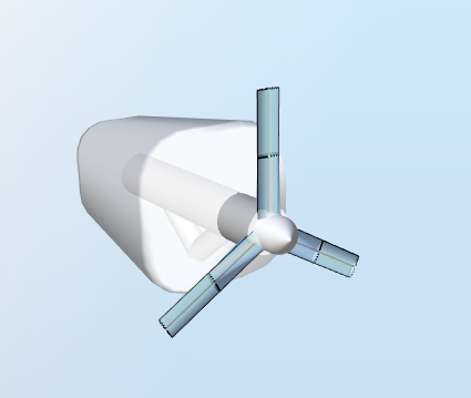
The chordlength accross the blade is  , the blade length is  and the hub radius is  .

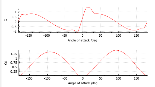
The blade used for this model has three Blade aerodynamical station  . The innermost station is at the root and has a cylindrical airfoil with no drag and no lift . This station will therefore not produce any aerodynamic loads. The two other blade aerodynamical stations have the NACA64-618 airfoil , which polar can be exported from Ashes and are shown in the figure below:

This test uses two variants of this blade:

• one variant has no twist (when the pitch is 0, the chordline of each blade station is in the rotor plane)
• one variant has twist, as shown in the table below

The table below gives a summary of the relevant blade characteristics:

Blade aerodynamical station	Distance to blade root	Influence length	Airfoil	Twist (if applicable)
1	$$r_1 = 0$$	$$L_{I1} = 1.25\text{ m}$$	Cylinder with no lift and drag	$$\theta = 0$$
2	$$r_2 = 2.5\text{ m}$$	$$L_{I2} = 2.5\text{ m}$$	NACA64-618	$$\theta = 20\text{ deg}$$
3	$$r_3 = 5\text{ m}$$	$$L_{I3}=1.25\text{ m}$$	NACA64-618	$$\theta = 5\text{ deg}$$

The air density is  . No gravity forces are applied, and tip and hub corrections are set to 0. The simulations are run in Loads only mode (see Analysis ), so the blade will not experience deflections and the rotational speed will not vary.

The wind speed and rotational speed are denoted   and  , respectively.

In order to compute the aerodynamic loads, we need to find the lift and drag coefficients for a given blade station. We do this using the steady BEM algorithm defined by  Hansen (2008d)  and summed up below:

1. define initial axial and tangential induced velocities as 
   $$a = 0.33$$
    and 
   $$a_t = 0$$
   , respectively
2. the flow angle is defined as 
   $$\phi = \tan^{-1}\frac{(1-a)\cdot V}{(1+a_t)\cdot\omega\cdot(r+r_h)}$$
3. the angle of attack is obtained by substracting the twist 
   $$\theta$$
    and the pitch
   $$\gamma$$
   to the flow angle. The angle of attack is thus 
   $$\alpha = \phi-\theta-\gamma$$
4. the lift and drag coefficients 
   $$C_L$$
    and
   $$C_D$$
   are then looked up from the polars. Linear interpolation is used if the current angle of attack is not in the look-up table.
5. the blade solidity is calculated as 
   $$\sigma = \frac{cB}{2\pi(r+r_h)}$$
   , where 
   $$B = 1$$
   is the number of blades
6. new values for the induced velocities are computed as
   
   $$a = \frac{1}{\frac{4\sin^2\phi}{\sigma C_n}+1}$$
   and
   
   $$a_t = \frac{1}{\frac{4\sin\phi\cos\phi}{\sigma C_t}+1}$$
   
   where 
   $$C_n = C_L\cos\phi+C_D\sin\phi$$
   and 
   $$C_t = C_L\sin\phi - C_D\cos\phi$$
7. compare the induced velocities to the previous values. If the difference is larger than 0.001, repeat steps 2 to 6
8. the relative velocity is defined as 
   $$V_{rel}=\sqrt{((1-a)\cdot V)^2+((1+a_t)\cdot\omega\cdot(r+r_h))^2}$$
9. the lift and drag forces, for blade station 
   $$i$$
   are then
   
   $$F_{D,i} = \frac{1}{2}\rho cC_DV_{rel}^2$$
   and
   
   $$F_{L,i} = \frac{1}{2}\rho cC_LV_{rel}^2$$
   
   
10. the thust and torque forces are then
    
    $$F_{th,i} = F_{L,i}\cos\phi+F_{D,i}\sin\phi$$
    and
    
    $$F_{t,i} = -F_{D,i}\cos\phi + F_{L,i}\sin\phi$$

The next three output are part of the  Blade [Time] sensor  sensor. The  root force is the sum of the drag and the lift forces from both stations, which can be expressed as  . The in-plane bending moment  is  and the out-of-plane bending moment  is 

This derivation is used for all the load cases run in this test. The table below sums up the expected results.

Test name	Description	Aerodynamic thrust  $$[\text{N}]$$	Aerodynamic torque   $$[\text{Nm}]$$	Root force   $$[\text{N}]$$	In plane bending moment   $$[\text{Nm}]$$	Out of plane bending moment   $$[\text{Nm}]$$	Cl  $$[\text{-}]$$	Cd  $$[\text{-}]$$
10 ms	Wind speed = 10 RPM = 5	305.4	37.64	305.6	32.72	1030	0.2804	1.3854
5 ms	Wind speed = 5 RPM = 5	81.22	8.859	81.25	7.708	278.3	0.4660	1.266
10 ms RPM 10	Wind speed = 10 RPM = 10	324.9	35.44	325.0	30.83	1113	0.4660	1.266
10 ms pitch 20	Wind speed = 10 RPM = 5 Pitch angle  = 20	255.4	387.0	274.4	336.8	857.9	0.6608	1.062
5 ms pitch 20	Wind speed = 5 RPM = 5 Pitch angle = 20	65.65	99.48	70.46	86.68	222.5	0.7556	0.8831
10 ms RPM 10 pitch 20	Wind speed = 10 RPM = 10 Pitch angle  = 20	262.6	397.9	281.9	346.7	890.2	0.7556	0.8831
10 ms twist	Wind speed = 10 RPM = 5 Blade with twist	270.9	264.4	282.0	225.3	935.4	0.6608	1.062
5 ms twist	Wind speed = 5 RPM = 5 Blade with twist	71.16	67.40	73.86	57.52	250.1	0.7556	0.8831
10 ms RPM 10 twist	Wind speed = 10 RPM = 10 Blade with twist	284.7	269.6	295.4	230.1	1000	0.7556	0.8831

4 Results

A simulation of ten seconds is run. The test is considered passed if the last two seconds of the results produced by Ashes lie within 1% of the analytical solution.

The report with the results can be found here:

https://www.simis.io/downloads/open/benchmarks/current/One airfoil blade.pdf