Nonlinear spring test
1 Test description
This test uses a model composed of two nodes and one element. One node is attached to a
nonlinear spring
(see
Nonlinear springs). A force is applied to that node and the node displacement is observed. A
erodynamic loads
and
gravity loads
are disabled. The model has a very low mass (5 g) so that its inertia is very low.
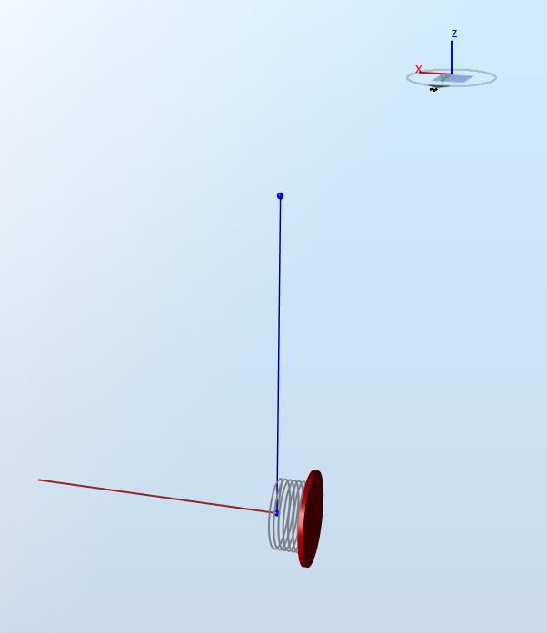
The figure below illustrates the model with a spring in the x-direction. The red vector represents a force in the x-direction.
2 Analytical solution
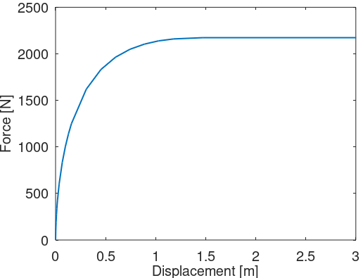
For this example, we use a force-displacement look-up table defined as follows:
$$d = [0,0.001846,0.003032,0.005129,0.008935,0.012521,0.015992,0.01939,0.035788,0.067292,0.098047,0.128399,0.158489,0.306783,0.453235,0.598768,0.743759,0.8884,1.03,1.18,1.47,144.03]$$
$$ Fs = [0,97.16,137.33,194.02,273.83,334.71,385.72,430.4,602.7,835.96,1004.52,1138.44,1249.68,1620.03,1831.5,1963.77,2049.2,2104.48,2139.39,2160.04,2173.5,2173.5]$$
This gives the following curve:
When a load is applied on to the node, the node is displaced by a certain amount. The system will reach equilibrium once the reaction force from the nonlinear spring is equal to the applied force. This implies that the node displacement will correspond to the value of the applied force.
If displacement values do not correspond to values given in the look-up table, a linear interpolation is performed.
For a given displacement
$$dx$$
such that
$$d_i \leq d_x < d_{i+1}$$
, the stiffnes as output in the
Support sensor is given by
$$K(d_x)=\frac{F_{i+1}-F_i}{d_{i+1}-d_i}$$
The first 7 load cases are static pull tests, where a constant force is applied onto the node until the displacement is stabilised. The table below gives the force applied in each load case and the expected displacement. The subscript x-y-z indicates the direction of the force and the displacement.
| Load case |
Force
$$[\text{N}]$$
|
Expected displacement
$$[\text{m}]$$
|
Expected stiffness
$$[\text{N}\cdot\text{m}^{-1}]$$ |
| x-direction 1000 N |
$$F_x = 1000$$
|
$$d_x = 0.0972$$
|
$$K_x=5480$$
|
| x-direction -200 N |
$$F_x = -200$$
|
$$d_x=-0.00541$$
|
$$K_x=21000$$
|
| y-direction 1000 N |
$$F_y=1000$$
|
$$d_y = 0.0972$$
|
$$K_y = 5480$$
|
| y-direction -300 N |
$$F_y = -300$$
|
$$d_y=-0.0105$$
|
$$K_y = 17000$$
|
| z-direction 500 N |
$$F_z = 500$$
|
$$d_z = 0.0260$$
|
$$K_z = 10500$$
|
| z-direction -1000 N |
$$F_z = -1000$$
|
$$d_z=-0.0972$$
|
$$K_z = 5480$$
|
| xy-direction |
$$F_x = 700\text{, }F_y = 800$$
|
$$d_x = 0.0489\text{, }d_y=0.0624$$
|
$$K_x = 7400\text{, }K_y = 7400$$
|
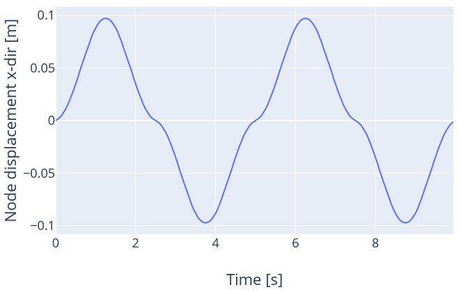
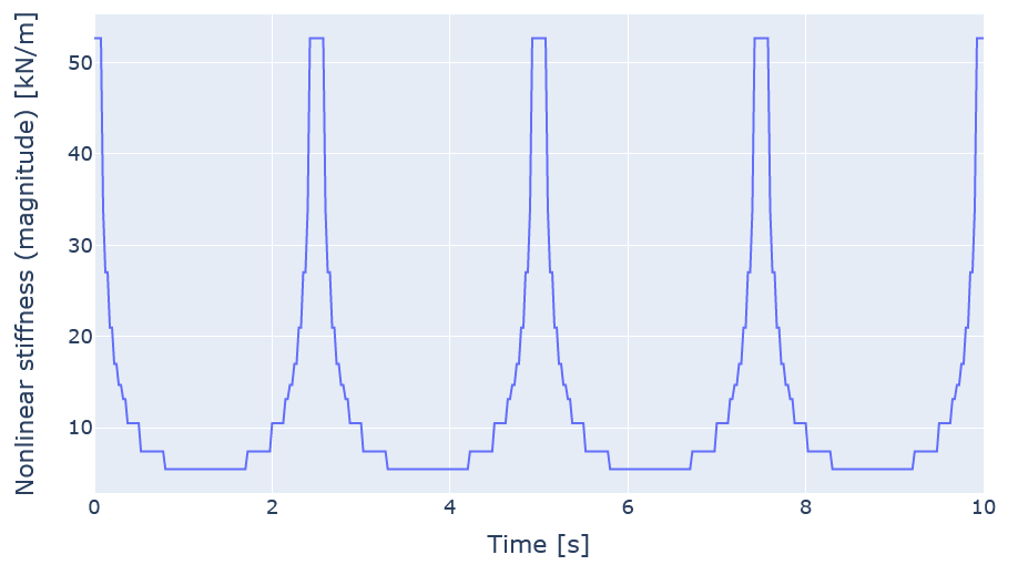
In the last load case, a sine force of amplitude 1000 N and period 5 sec is applied onto the load. The mass of the model is very low so that the eigenfrequency is virtually infinite. This implies that the node will reach its static position virtually instantly for each time step (see for example
Biggs (1964)). We can this find the expected stiffness and displacement corresponding to the force applied at each time step. The expected node displacement and stiffness will be as illustrated in the figures below:
3 Results
In Ashes, the loads are applied with a
ramp-up, i.e. they start at 0 and are progressively increased until their value (see
Analysis). Therefore, the output produced by Ashes will show a ramp-up period as well.
A test is considered passed when all values of the last two seconds of the results produced by Ashes are within 0.1% of the analytical solution. For the last load case, because the values of the node displacement can take very small values, the relative difference between Ashes and the analytical solution can be relatively large. A limit of 2% is taken for this load case.
The report for this test can be found on the following link: