Note: the inertia coefficient
$$C_M$$
is also sometimes called
Mass coefficient. It is different from the
added mass coefficient, generally noted
$$C_m$$
or
$$C_a$$
. The link between the mass coefficient and the added mass coefficient is
$$C_M = 1+C_m$$
.
$$C_m$$
is generaly between 0.5 and 1, which means that
$$C_M$$
is generally between 1.5 and 2.
1.2
Heave plates
Heave plates need to be treated differently when it comes to the added mass considerations because the force on a heave plate does not scale with the volume of displaced fluid. The added mass force on a heave plate is computed as
$$F_{hydro}= \frac{1}{2}\rho C_D\pi R^2\mid w-\dot z \mid(w-\dot z) + \rho C_M\frac{4}{3}\pi R^3a_z-\rho\cdot (C_M-1)\frac{4}{3}\pi R^3\ddot{z}$$
where
$$\ddot{z}$$
is the vertical acceleration of the heave plate.
Note: the added mass force described above is not a distributed force, contrary to the different terms of the
Transverse flow
forces.
2
Application of the force to the structural model
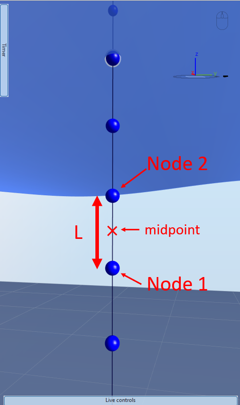
The Morison equation is quite simple, however it is not trivial to apply it to a finite element model because loads can only be applied to nodes, therefore assumptions have to be made on how distributed loads are lumped onto nodes. This section explains how this is done in Ashes by considering the element defined by nodes 1 and 2 in the figure below:
The coordinates of Node 1, Node 2 and the midpoint are respectively
$$z_1$$
,
$$z_2$$
and
$$z_{12}$$
. Note that
$$z_{12} = 0.5(z_1+z_2)$$
.
We separate the Morison equation into three contributions: a
drag
term
$$F_D$$
, a
mass term
$$F_M$$
and an
added mass term
$$F_a$$
. In the present example, the drag and mass terms at node 1 will be
$$F_{D,1} = \rho C_DR\frac{L}{2}\mid u(z_{12})-\dot x(z_{12}) \mid(u(z_{12})-\dot x(z_{12})) $$
and
$$F_{M,1}=\rho C_M\pi R^2\frac{L}{2}a(z_{12}) $$
The drag and mass forces applied to node 2 will be defined in the same way, such that
$$F_{D,1} = F_{D,2}$$
and
$$F_{M,1} = F_{M,2}$$
.
Note: this implies that node 1 will have
two drag forces and
two mass forces applied to it: one pair of drag + mass forces will come from the element considered in this example (i.e. the element above node 1) and one pair will come from the element below node 1.
Similarly, node 2 will also have two drag forces and two mass forces.
This will not be the cases for nodes that are only connected to one element (for example the lowest node of a monopile) or nodes that are connected to an element that does not experience hydrodynamic loads.
The added mass term on node 1 will be
$$F_{a,1} = -\rho(C_M-1)\pi R^2\frac{L}{2}\ddot x(z_1)$$
and the added mass on node 2 will be
$$F_{a,2} = -\rho(C_M-1)\pi R^2\frac{L}{2}\ddot x(z_2)$$
For the added mass term, since the acceleration of the structure is taken at the node, the force can be different at the two nodes.
Note that it is possible to define an
added mass
$$m_a = -\rho(C_M-1)\pi R^2 L/2$$
, in which case the added mass force can be written as
$$F_{a,i} = m_a\ddot x(z_2)$$
In the equation of motion described in the
Time domain simulation document, the drag and mass forces
$$F_D$$
and
$$F_M$$
are computed as
external forces (i.e. on the right-hand side of the equation) and the added mass force
$$F_a$$
is computed by including the added mass
$$m_a$$
as a mass in the left-hand side of the equation. This is done so that the added mass is taken into account when computing the eigenmodes of a model.
The
Morison test provides a good illustration of how the Morison loads are computed and applied to a monopile. In this test, the structure is considered infinitely stiff, which means that it cannot move and that the added mass term will be 0.