Unsteady BEM
The unsteady BEM accounts for the dynamic variations of the relative velocity at the blade element, which can be produced by
- a rotating rotor with yaw/tilt/cone angles or in a non-spatially uniform wind (for example with shear)
- the controller pitching the blades or accelerating/decelerating the rotor
- the vibration of the blades or the motion of the tower
- turbulent wind
$$t=t_n$$
based on the wind conditions at system position at
$$t_n$$
and the induced velovity at the previous time step
$$t=t_{n-1}$$
.
Note: at t = 0, since no previous time step is available, the induced velocity is calculated with the
Steady BEM algorithm even if the Unsteady BEM scheme is selected. The ensuing time steps are computed with the Unsteady BEM
The computation of the induced velocity at a time step
$$t_n$$
is done performing the following steps:1 Calculate the relative velocity and the angle of attack
The relative velocity is taken as the sum of the wind velocity, the rotational velocity of the element and the induced velocity of the previous time step
$$t=t_{n-1}$$
, noted
$$W_{i,n-1}$$
. The angle of attack is then calculated following step 2 of the
Steady BEM algorithm, as illustrated in the figure below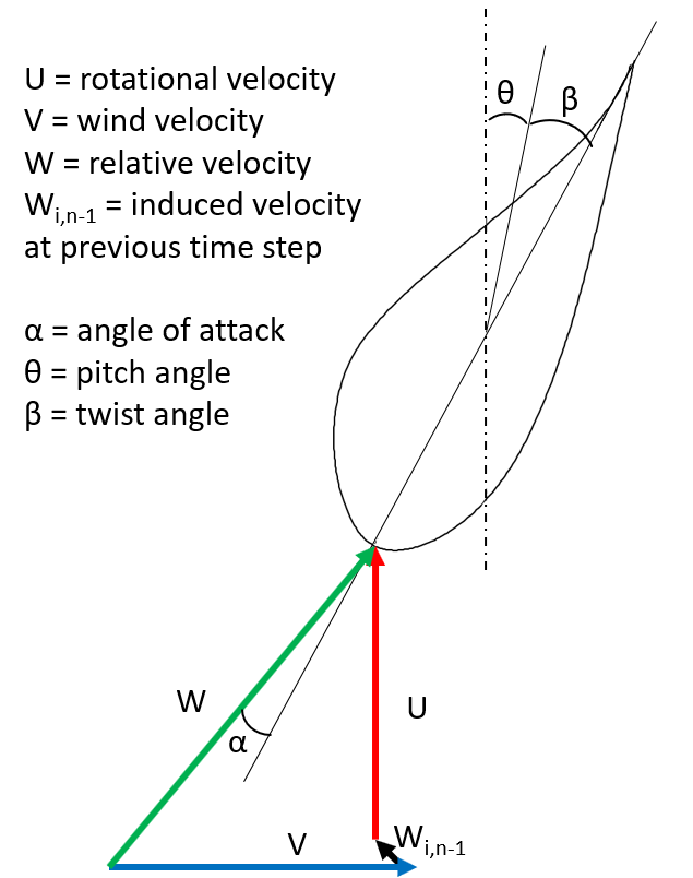
2 Compute the aerodynamic coefficients accounting for dynamic stall
First, the Reynolds number is calculated and the aerodynamic coefficients are looked up from the
Airfoil polar file, as in step 3 of the
Steady BEM algorithm.
Two options can be selected to take into account dynamic stall effects:
- Oye's dynamic stall model
- Oye's dynamic stall model
3 Calculate the quasi-static induced velocity
Once the aerodynamic coefficients have been calculated and adjusted for dynamic stall, the lift and drag forces are computed as in step 4 of the
Steady BEM algorithm, and a quasi-static induced velocity
$$W_{qs,n}$$
is computed from those forces as in step 5 of the
Steady BEM.
If requested in the
Aerodynamics tab of the
Analysis parameters window, this steps will include tip and hub loss correction based on Prandlt's factor and Glauert correction.
4 Compute the dynamic induced velocity
Based on the quasi-static induced velocity, a dynamic induced velocity is calculated following the equations presented in
Hansen (2008d). Two time constants are defined such as
$$\tau_1=\frac{1.1}{1-1.3a}\cdot\frac{R}{|V|}$$
and
$$\tau_2=\left(0.39-0.26\left(\frac{r}{R}\right)^2\right)\cdot\tau_1$$
where
$$a$$
is the axial induction factor based on the induced velocity at the previous time step and the current wind speed,
$$R$$
is the rotor radius,
$$|V|$$
is the magnitude of the wind velocity and
$$r$$
is the distance from the current element to the axis of rotation of the rotor.
Note: if
$$a>0.5$$
, the value
$$a=0.5$$
is used instead
The dynamic induced velocity at the time
$$t=t_n$$
is then given by
$$W_{i,n}+\tau_2\frac{dW_{i,n}}{dt}=W_{int,n}$$
where
$$W_{int,n}$$
is an intermediate value of
$$W_{i,n}$$
dependent on the quasi-static induced velocity through the following equation:
$$W_{int,n}+\tau_1\frac{dW_{int,n}}{dt}=W_{qs,n}+k\cdot\tau_1\frac{dW_{qs,n}}{dt}$$
with
$$k=0.6$$
.
Note: according to Martin Hansen (author of the book on which these equations are based), the value of
$$k$$
"is empirically calibrated to fit measurements, and maybe this value should be different for the very large WTs being build now." (Jan-2024)
In practice, this equations are solved assuming that their right-hand sides are constant and taking the values at time step
$$t=t_{n-1}$$
. The right-hand side of the previous equation is given by
$$H=W_{qs,n}+k\cdot\tau_1\frac{W_{qs,n}-W_{qs,n-1}}{\Delta t}$$
where
$$\Delta t=t_{n}-t_{n-1}$$
. Then,
$$W_{int,n}$$
is obained analytically through
$$W_{int,n}=H+(W_{int,n}-H)\exp{\left(-\frac{\Delta t}{\tau_1}\right)}$$
$$W_{i,n}$$
is then obtained analytically through
$$W_{i,n}=W_{int,n}+(W_{i,n-1}-W_{int,n})\cdot\exp{\left(-\frac{\Delta t}{\tau_2}\right)}$$
C
L
=
f
s
C
L
,
i
n
v
(
α
)
+
(
1
−
f
s
)
C
L
,
f
s
(
α
)
C
L
=
f
s
C
L
,
i
n
v
(
α
)
+
(
1
−
f
s
)
C
L
,
f
s
(
α
)
C
L
=
f
s
C
L
,
i
n
v
(
α
)
+
(
1
−
f
s
)
C
L
,
f
s
(
α
)
C
L
=
f
s
C
L
,
i
n
v
(
α
)
+
(
1
−
f
s
)
C
L
,
f
s
(
α
)
C
L
=
f
s
C
L
,
i
n
v
(
α
)
+
(
1
−
f
s
)
C
L
,
f
s
(
α
)
C
L
=
f
s
C
L
,
i
n
v
(
α
)
+
(
1
−
f
s
)
C
L
,
f
s
(
α
)
C
L
=
f
s
C
L
,
i
n
v
(
α
)
+
(
1
−
f
s
)
C
L
,
f
s
(
α
)
C
L
=
f
s
C
L
,
i
n
v
(
α
)
+
(
1
−
f
s
)
C
L
,
f
s
(
α
)
C
L
=
f
s
C
L
,
i
n
v
(
α
)
+
(
1
−
f
s
)
C
L
,
f
s
(
α
)
C
L
=
f
s
C
L
,
i
n
v
(
α
)
+
(
1
−
f
s
)
C
L
,
f
s
(
α
)
C
L
=
f
s
C
L
,
i
n
v
(
α
)
+
(
1
−
f
s
)
C
L
,
f
s
(
α
)
C
L
=
f
s
C
L
,
i
n
v
(
α
)
+
(
1
−
f
s
)
C
L
,
f
s
(
α
)
C
L
=
f
s
C
L
,
i
n
v
(
α
)
+
(
1
−
f
s
)
C
L
,
f
s
(
α
)
C
L
=
f
s
C
L
,
i
n
v
(
α
)
+
(
1
−
f
s
)
C
L
,
f
s
(
α
)
C
L
=
f
s
C
L
,
i
n
v
(
α
)
+
(
1
−
f
s
)
C
L
,
f
s
(
α
)
C
L
=
f
s
C
L
,
i
n
v
(
α
)
+
(
1
−
f
s
)
C
L
,
f
s
(
α
)
C
L
=
f
s
C
L
,
i
n
v
(
α
)
+
(
1
−
f
s
)
C
L
,
f
s
(
α
)
C
L
=
f
s
C
L
,
i
n
v
(
α
)
+
(
1
−
f
s
)
C
L
,
f
s
(
α
)
C
L
=
f
s
C
L
,
i
n
v
(
α
)
+
(
1
−
f
s
)
C
L
,
f
s
(
α
)
C
L
=
f
s
C
L
,
i
n
v
(
α
)
+
(
1
−
f
s
)
C
L
,
f
s
(
α
)
C
L
=
f
s
C
L
,
i
n
v
(
α
)
+
(
1
−
f
s
)
C
L
,
f
s
(
α
)
C
L
=
f
s
C
L
,
i
n
v
(
α
)
+
(
1
−
f
s
)
C
L
,
f
s
(
α
)
C
L
=
f
s
C
L
,
i
n
v
(
α
)
+
(
1
−
f
s
)
C
L
,
f
s
(
α
)
C
L
=
f
s
C
L
,
i
n
v
(
α
)
+
(
1
−
f
s
)
C
L
,
f
s
(
α
)
C
L
=
f
s
C
L
,
i
n
v
(
α
)
+
(
1
−
f
s
)
C
L
,
f
s
(
α
)
C
L
=
f
s
C
L
,
i
n
v
(
α
)
+
(
1
−
f
s
)
C
L
,
f
s
(
α
)
C
L
=
f
s
C
L
,
i
n
v
(
α
)
+
(
1
−
f
s
)
C
L
,
f
s
(
α
)
C
L
=
f
s
C
L
,
i
n
v
(
α
)
+
(
1
−
f
s
)
C
L
,
f
s
(
α
)
C
L
=
f
s
C
L
,
i
n
v
(
α
)
+
(
1
−
f
s
)
C
L
,
f
s
(
α
)
C
L
=
f
s
C
L
,
i
n
v
(
α
)
+
(
1
−
f
s
)
C
L
,
f
s
(
α
)
C
L
=
f
s
C
L
,
i
n
v
(
α
)
+
(
1
−
f
s
)
C
L
,
f
s
(
α
)
C
L
=
f
s
C
L
,
i
n
v
(
α
)
+
(
1
−
f
s
)
C
L
,
f
s
(
α
)
C
L
=
f
s
C
L
,
i
n
v
(
α
)
+
(
1
−
f
s
)
C
L
,
f
s
(
α
)
C
L
=
f
s
C
L
,
i
n
v
(
α
)
+
(
1
−
f
s
)
C
L
,
f
s
(
α
)
C
L
=
f
s
C
L
,
i
n
v
(
α
)
+
(
1
−
f
s
)
C
L
,
f
s
(
α
)
C
L
=
f
s
C
L
,
i
n
v
(
α
)
+
(
1
−
f
s
)
C
L
,
f
s
(
α
)
C
L
=
f
s
C
L
,
i
n
v
(
α
)
+
(
1
−
f
s
)
C
L
,
f
s
(
α
)
C
L
=
f
s
C
L
,
i
n
v
(
α
)
+
(
1
−
f
s
)
C
L
,
f
s
(
α
)
C
L
=
f
s
C
L
,
i
n
v
(
α
)
+
(
1
−
f
s
)
C
L
,
f
s
(
α
)
C
L
=
f
s
C
L
,
i
n
v
(
α
)
+
(
1
−
f
s
)
C
L
,
f
s
(
α
)
C
L
=
f
s
C
L
,
i
n
v
(
α
)
+
(
1
−
f
s
)
C
L
,
f
s
(
α
)
C
L
=
f
s
C
L
,
i
n
v
(
α
)
+
(
1
−
f
s
)
C
L
,
f
s
(
α
)
C
L
=
f
s
C
L
,
i
n
v
(
α
)
+
(
1
−
f
s
)
C
L
,
f
s
(
α
)
C
L
=
f
s
C
L
,
i
n
v
(
α
)
+
(
1
−
f
s
)
C
L
,
f
s
(
α
)
C
L
=
f
s
C
L
,
i
n
v
(
α
)
+
(
1
−
f
s
)
C
L
,
f
s
(
α
)
C
L
=
f
s
C
L
,
i
n
v
(
α
)
+
(
1
−
f
s
)
C
L
,
f
s
(
α
)
C
L
=
f
s
C
L
,
i
n
v
(
α
)
+
(
1
−
f
s
)
C
L
,
f
s
(
α
)
C
L
=
f
s
C
L
,
i
n
v
(
α
)
+
(
1
−
f
s
)
C
L
,
f
s
(
α
)
C
L
=
f
s
C
L
,
i
n
v
(
α
)
+
(
1
−
f
s
)
C
L
,
f
s
(
α
)
C
L
=
f
s
C
L
,
i
n
v
(
α
)
+
(
1
−
f
s
)
C
L
,
f
s
(
α
)
C
L
=
f
s
C
L
,
i
n
v
(
α
)
+
(
1
−
f
s
)
C
L
,
f
s
(
α
)
C
L
=
f
s
C
L
,
i
n
v
(
α
)
+
(
1
−
f
s
)
C
L
,
f
s
(
α
)
C
L
=
f
s
C
L
,
i
n
v
(
α
)
+
(
1
−
f
s
)
C
L
,
f
s
(
α
)
C
L
=
f
s
C
L
,
i
n
v
(
α
)
+
(
1
−
f
s
)
C
L
,
f
s
(
α
)
C
L
=
f
s
C
L
,
i
n
v
(
α
)
+
(
1
−
f
s
)
C
L
,
f
s
(
α
)
C
L
=
f
s
C
L
,
i
n
v
(
α
)
+
(
1
−
f
s
)
C
L
,
f
s
(
α
)
C
L
=
f
s
C
L
,
i
n
v
(
α
)
+
(
1
−
f
s
)
C
L
,
f
s
(
α
)
C
L
=
f
s
C
L
,
i
n
v
(
α
)
+
(
1
−
f
s
)
C
L
,
f
s
(
α
)
C
L
=
f
s
C
L
,
i
n
v
(
α
)
+
(
1
−
f
s
)
C
L
,
f
s
(
α
)
C
L
=
f
s
C
L
,
i
n
v
(
α
)
+
(
1
−
f
s
)
C
L
,
f
s
(
α
)
C
L
=
f
s
C
L
,
i
n
v
(
α
)
+
(
1
−
f
s
)
C
L
,
f
s
(
α
)
C
L
=
f
s
C
L
,
i
n
v
(
α
)
+
(
1
−
f
s
)
C
L
,
f
s
(
α
)
C
L
=
f
s
C
L
,
i
n
v
(
α
)
+
(
1
−
f
s
)
C
L
,
f
s
(
α
)
C
L
=
f
s
C
L
,
i
n
v
(
α
)
+
(
1
−
f
s
)
C
L
,
f
s
(
α
)
C
L
=
f
s
C
L
,
i
n
v
(
α
)
+
(
1
−
f
s
)
C
L
,
f
s
(
α
)
C
L
=
f
s
C
L
,
i
n
v
(
α
)
+
(
1
−
f
s
)
C
L
,
f
s
(
α
)
C
L
=
f
s
C
L
,
i
n
v
(
α
)
+
(
1
−
f
s
)
C
L
,
f
s
(
α
)
C
L
=
f
s
C
L
,
i
n
v
(
α
)
+
(
1
−
f
s
)
C
L
,
f
s
(
α
)
C
L
=
f
s
C
L
,
i
n
v
(
α
)
+
(
1
−
f
s
)
C
L
,
f
s
(
α
)
C
L
=
f
s
C
L
,
i
n
v
(
α
)
+
(
1
−
f
s
)
C
L
,
f
s
(
α
)
C
L
=
f
s
C
L
,
i
n
v
(
α
)
+
(
1
−
f
s
)
C
L
,
f
s
(
α
)
C
L
=
f
s
C
L
,
i
n
v
(
α
)
+
(
1
−
f
s
)
C
L
,
f
s
(
α
)
C
L
=
f
s
C
L
,
i
n
v
(
α
)
+
(
1
−
f
s
)
C
L
,
f
s
(
α
)
C
L
=
f
s
C
L
,
i
n
v
(
α
)
+
(
1
−
f
s
)
C
L
,
f
s
(
α
)
C
L
=
f
s
C
L
,
i
n
v
(
α
)
+
(
1
−
f
s
)
C
L
,
f
s
(
α
)
C
L
=
f
s
C
L
,
i
n
v
(
α
)
+
(
1
−
f
s
)
C
L
,
f
s
(
α
)
C
L
=
f
s
C
L
,
i
n
v
(
α
)
+
(
1
−
f
s
)
C
L
,
f
s
(
α
)
C
L
=
f
s
C
L
,
i
n
v
(
α
)
+
(
1
−
f
s
)
C
L
,
f
s
(
α
)
C
L
=
f
s
C
L
,
i
n
v
(
α
)
+
(
1
−
f
s
)
C
L
,
f
s
(
α
)
C
L
=
f
s
C
L
,
i
n
v
(
α
)
+
(
1
−
f
s
)
C
L
,
f
s
(
α
)
C
L
=
f
s
C
L
,
i
n
v
(
α
)
+
(
1
−
f
s
)
C
L
,
f
s
(
α
)
C
L
=
f
s
C
L
,
i
n
v
(
α
)
+
(
1
−
f
s
)
C
L
,
f
s
(
α
)
C
L
=
f
s
C
L
,
i
n
v
(
α
)
+
(
1
−
f
s
)
C
L
,
f
s
(
α
)
C
L
=
f
s
C
L
,
i
n
v
(
α
)
+
(
1
−
f
s
)
C
L
,
f
s
(
α
)
C
L
=
f
s
C
L
,
i
n
v
(
α
)
+
(
1
−
f
s
)
C
L
,
f
s
(
α
)
C
L
=
f
s
C
L
,
i
n
v
(
α
)
+
(
1
−
f
s
)
C
L
,
f
s
(
α
)
C
L
=
f
s
C
L
,
i
n
v
(
α
)
+
(
1
−
f
s
)
C
L
,
f
s
(
α
)
C
L
=
f
s
C
L
,
i
n
v
(
α
)
+
(
1
−
f
s
)
C
L
,
f
s
(
α
)
C
L
=
f
s
C
L
,
i
n
v
(
α
)
+
(
1
−
f
s
)
C
L
,
f
s
(
α
)
C
L
=
f
s
C
L
,
i
n
v
(
α
)
+
(
1
−
f
s
)
C
L
,
f
s
(
α
)
5 Apply the Yaw/Tilt factor
The Yaw/tilt model as described in step 7 of the
Steady BEM algorithm is then applied to the dynamic induced velocity.
6 Compute the aerodynamic loads
Once the induced velocity is known, the aerodynamic loads are calculated as in step 4 of the
Steady BEM algorithm assuming the aerodynamic coefficients calculated in step 2