Blade decay test
1 Test description
This test uses a blade with a constant cross section fixed onto the hub (i.e. behaving like a cantiliever beam). Gravity and aerodynamic loads are disabled. The model uses
Euler-Bernoulli elements.
This is a reproduction of
Decay test tower in order to verify that the structural implementation of the blades produces correct results. The model is therefore not meant to represent a realistic wind turbine blade.
The following load cases are tested
- Decay no damping
- Decay no damping stiffness x 2
- Decay no damping stiffness x 0.5
- Mass only
- Stiffness only
- Mass only 2nd mode
- Stiffness only 2nd mode
- Rayleigh first mode
- Rayleigh second mode
- Mass from coefficients
- Stiffness from coefficients
- Rayleigh from coefficients
2 Model
2.1 Model description
The model used for this test is shown in the figure below:
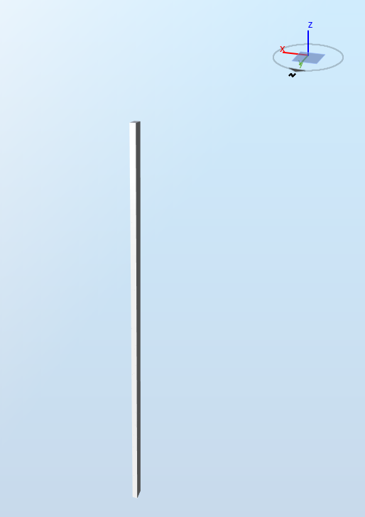
The blade has a constant cross section with in-plane and out-of-plane second moments of area equal to
$$I_x =3.276\cdot10^{-1}\text{ m}^4$$
and
$$I_y = 1.344\text{ m}^4$$
The length of the model is
$$l=87.6\text{ m}$$
., and the structure is divided into 200 elements.
The linear mass is
$$m=(bh-(b-2t)\cdot(h-2t))\cdot d=3539\text{ kg}\cdot\text{m}^{-1}$$
The material has an Elastic modulus
$$E=2.1\cdot10^{11}\text{ Pa}$$
The first and second eigenperiods of the structure are given by the following equations (
Biggs (1964)):
$$T_1 = \left(\frac{l}{0.597\pi}\right)^2\sqrt{\frac{m}{EI_x}}=3.109\text{ s}$$
and
$$T_2 = \left(\frac{l}{0.597\pi}\right)^2\sqrt{\frac{m}{EI_y}}=1.535\text{ s}$$
We note
$$\omega_1=2\pi/T1$$
and
$$\omega_2=2\pi/T_2$$
the two first eigenfrequencies of the structure.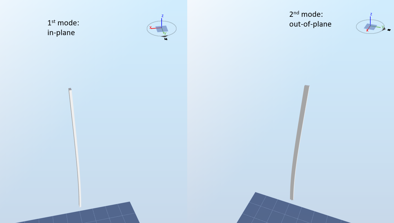
Note: for a typical blade, at 0 pitch, the in-plane mode corresponds to the edgewise mode, and the out-of-plane mode corresponds to the flapwise mode. In general, the flapwise mode has a lower eigenfrequency than the edgewise mode.
In this test, the elements are modeled as Euler-Bernoulli beams. No aerodynamic or gravity loads are applied to the model.
2.2 Initial conditions
For each load case, at the beginning of the simulation
$$t=0$$
, all nodes are constrained to move at a given velocity (and the constraint is then removed). The velocity applied at each node is scaled with the displacement of that node for a given mode shape, and normalized so that the maximum velocity is
$$1\text{ m}\cdot{s}^{-1}$$
. This ensures that the motion of the model will be purely harmonic, i.e. if the 1st mode shape is chosen to scale the velocities, only 1st mode motion will be observed in the simulation.3 Analytical solution
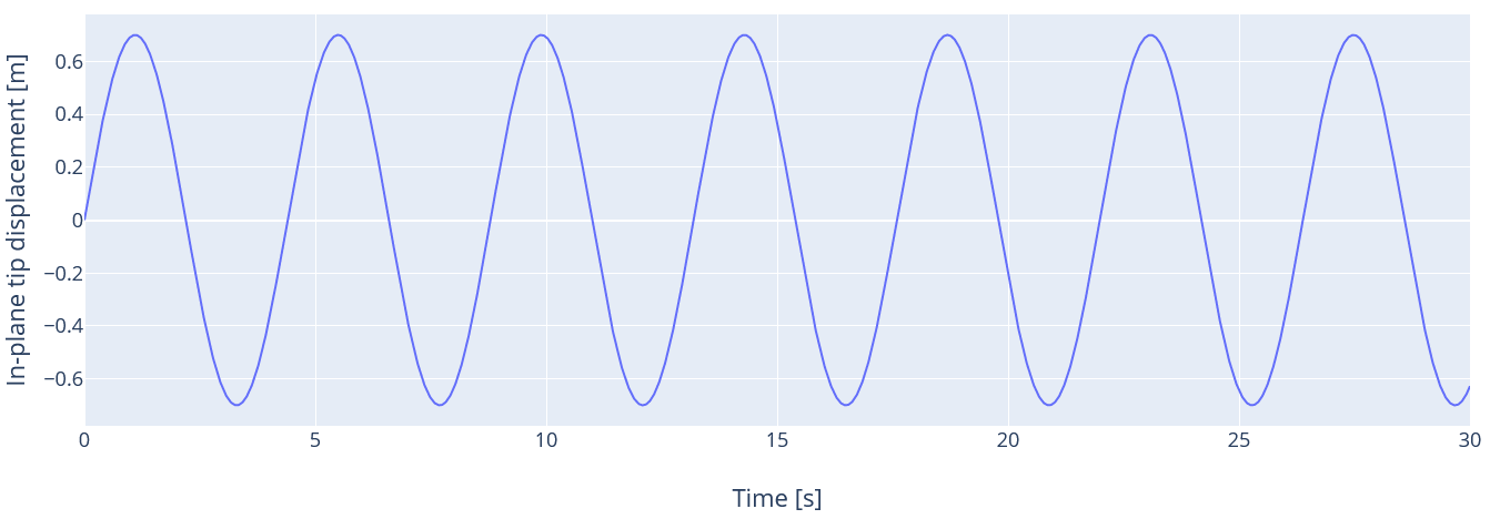
3.1 Decay no damping
in this load case, no damping is applied, and the first mode shape is used to define the initial conditions. The top node of the structure is the one that will experience maximum displacement, so the velocity at that node is expected to oscillate between
$$1\text{ m}\cdot{s}^{-1}$$
and
$$-1\text{ m}\cdot{s}^{-1}$$
with a period
$$T_1$$
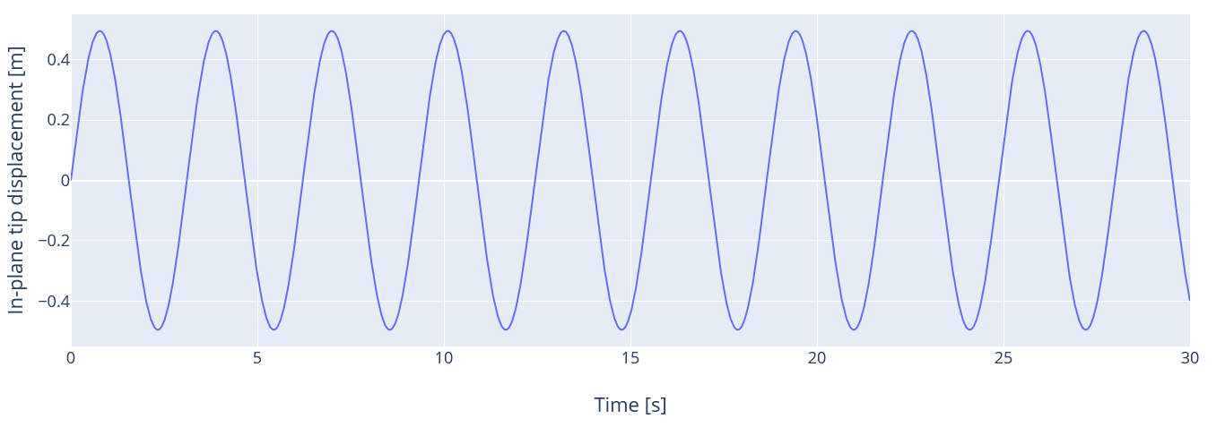
. The velocity of the top node is thus expected to vary as
$$v_y(t) = \cos(\omega_1t)$$
The expected displacement of the top node will thus be
$$d_y(t)=\frac{1}{\omega_1}\sin\left(\omega_1t\right)$$
The time series for the displacement is given in the figure below:
3.2 Decay no damping stiffness x 2
In this test, the stiffness of the blade is multiplied by 2, using the
Structural scale factor of the
Rotor part. This is equivalent to have an Elastic modulus twice as large as for the previous case.
3.3 Decay no damping stiffness x 0.5
In this test, the stiffness of the original blade is divided by 2.
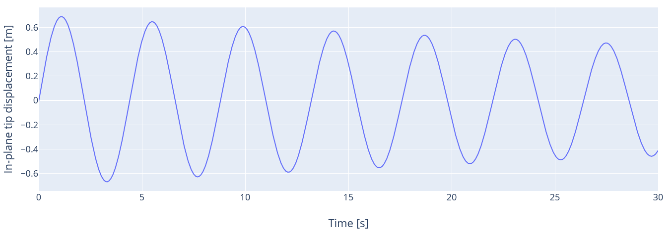
3.4 Mass only
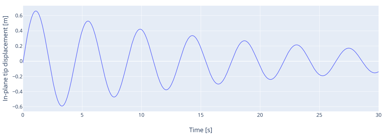
In this load case, we apply the mass term of Rayleigh damping (see
How to use Rayleigh damping). We set the damping ratio for the first mode
$$\xi_1$$
to be 1%, and we use the 1st mode as initial conditions. Therefore, we expect the velocity to decay as
$$v_y(t)=e^{-\xi_1\omega_1t}\cos(\omega_1t)$$
The expected displacement of the top node will thus be
$$d_y(t)=e^{-\xi_1\omega_1t}\frac{\sin(\omega_1t)-\xi_1\cos(\omega_1t)}{(\xi_1^2+1)\omega_1}$$
The time series for the displacement is given in the figure below:
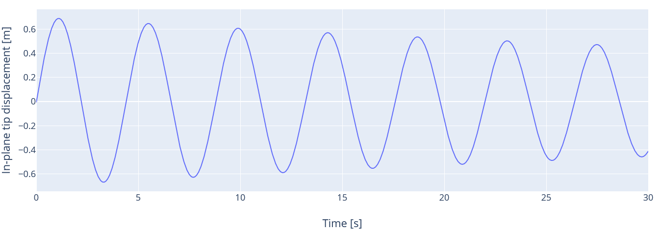
3.5 Stiffness only
This load case is similar to the previous one, but we use only the stiffness term of Rayleigh danping instead of the mass term. The damping ratio is still set to 1% for the first mode, thus we expect the same displacement as in the previous case.
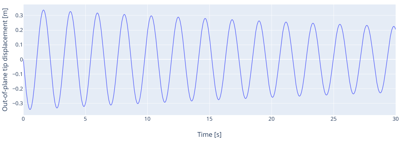
3.6 Mass only second mode
In this load case, we use the second mode shape as initial conditions. Therefore we only expect 2nd mode motion, and displacements will only be in the x-direction. The damping ratio for the first mode
$$\xi_1$$
is still 1%.
If only the mass term of Rayleigh damping is considered, the damping ratio for a given frequency
$$\omega$$
is given by
$$\xi(\omega)=0.5\frac{\mu}{\omega}$$
where
$$\mu$$
is the
mass coefficient (see
How to use Rayleigh damping). By inserting
$$\xi_1$$
and
$$\omega_1$$
in this equation, we find that the expected damping ratio for the second mode is
$$\xi_2 = \xi_1\frac{\omega_1}{\omega_2}=0.49\%$$
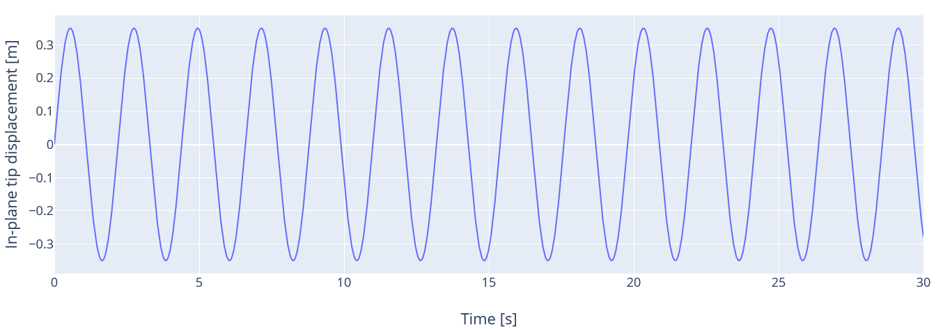
The expected displacement of the top node is thus
$$d_x(t)=e^{-\xi_2\omega_2t}\frac{\sin(\omega_2t)-\xi_2\cos(\omega_2t)}{(\xi_2^2+1)\omega_2}$$
The time series for the displacement is given in the figure below:
3.7 Stiffness only second mode
The same initial conditions as the previous case are used here. if only the stiffness term of Rayleigh damping is used, we have
$$\xi(\omega)=0.5\lambda\omega$$
Similarly to what was done in the previous load case, the expected damping ratio for the second mode is
$$\xi_2 = \xi_1\frac{\omega_2}{\omega_1}=2.0\%$$
The expected time series for the displacement is given in the figure below:
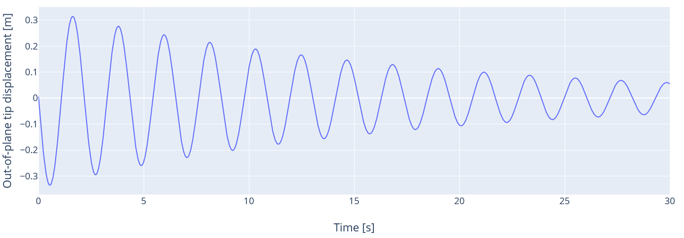
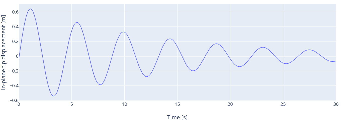
3.8 Rayleigh first mode
In this load case, we apply both the mass and stiffness terms, and we use the first mode as initial conditions. We set the parameters of Rayleigh damping such that the damping ratio for a period of 3 s is 1% and the ratio for a period of 0.3 s is 2%. We can then calculate the mass and stiffness coefficients (see
How to use Rayleigh damping):
$$\mu = 0.03384\text{ rad}\cdot\text{s}^{-1}$$
,
$$\lambda = 0.001833\text{ s}\cdot\text{rad}^{-1}$$
The damping ratio for the first mode is thus
$$\xi_1=0.5\left(\frac{\mu}{\omega_1}+\lambda\omega_1\right)=1.02\%$$
Therefore, we expect the top node dispoacement in the y-direction to be
$$d_y(t)=e^{-\xi_1\omega_1t}\frac{\sin(\omega_1t)-\xi_1\cos(\omega_1t)}{(\xi_1^2+1)\omega_1}$$
The time series for the displacement is given in the figure below:
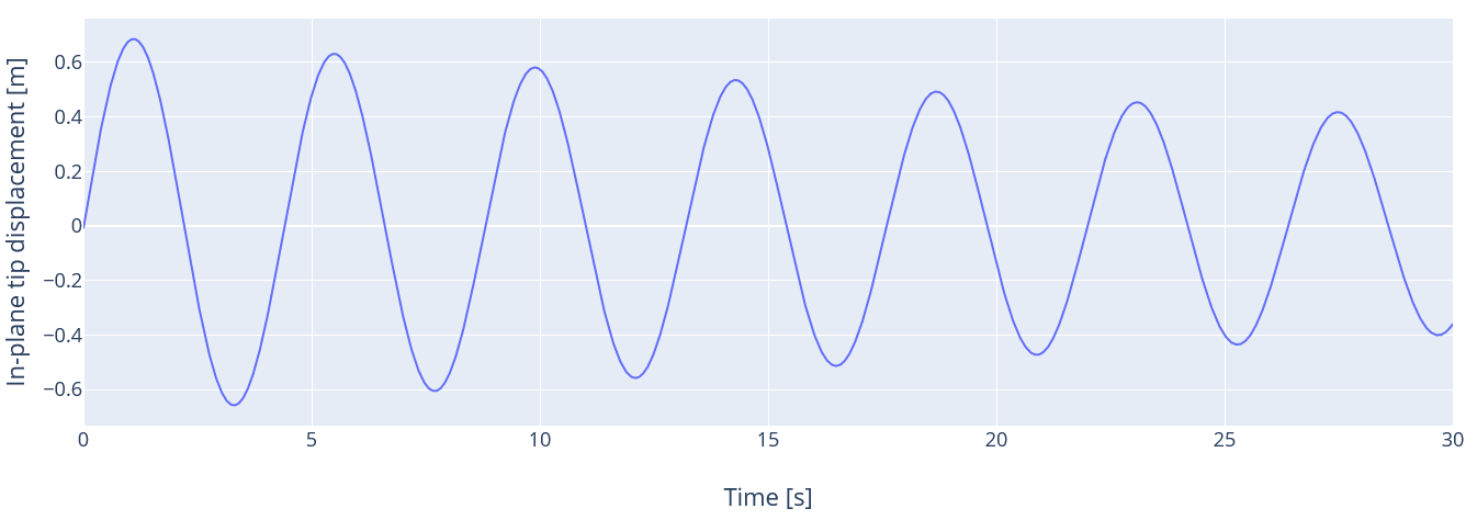
3.9 Rayleigh second mode
This load case is similar to the previous one, but the second mode is used for initial conditions. The damping ratio for the second mode will be
$$\xi_2=0.5\left(\frac{\mu}{\omega_2}+\lambda\omega_2\right)=0.79\%$$
The time series for the displacement is given in the figure below:
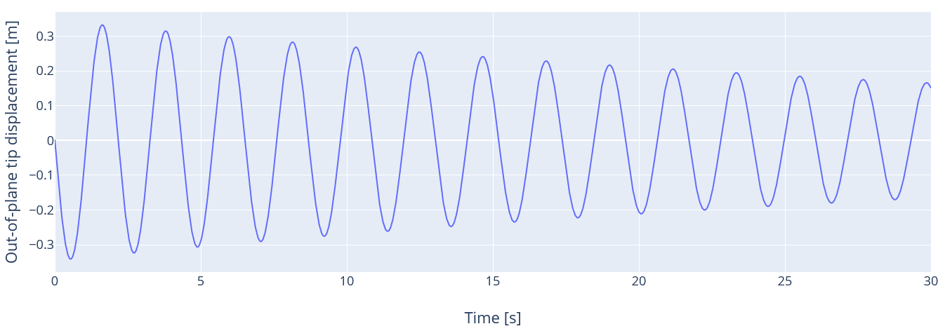
3.10 Mass from coefficients
In all the previous load cases, the input was a damping ratio and a corresponding period, and those inputs enabled the calculation of the mass and stiffness coefficients. It is also possoble to specify directly the coefficients. In this load case, we only consider the mass term and set the mass coefficient as
$$\mu = 0.05\text{ rad}\cdot\text{s}^{-1}$$
. We use te first mode as initial conditions.
The damping ratio for the first mode is then
$$\xi_1 = 0.5\frac{\mu}{\omega_1}=1.23\%$$
The time series for the displacement is given in the figure below:
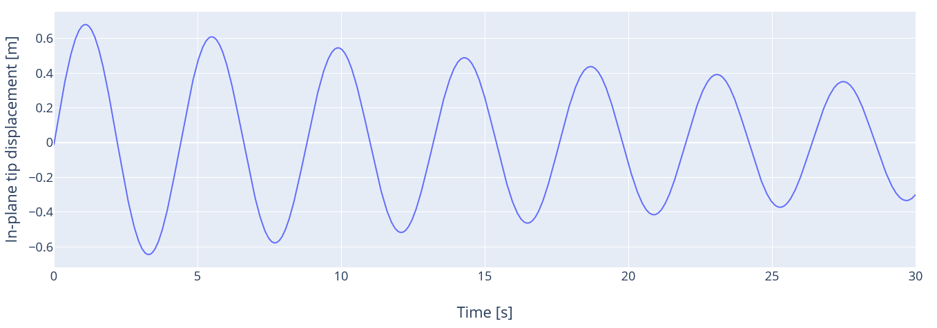
3.11 Stifness from coefficients
This load case is similar to the previous one but we only consider the stiffness term and set the stiffness coefficient as
$$\lambda = 0.05\text{ s}\cdot\text{rad}^{-1}$$
We use te first mode as initial conditions.
The damping ratio for the first mode is then
$$\xi_1 = 0.5\lambda{\omega_1}=5.05\%$$
The time series for the displacement is given in the figure below:
3.12 Rayleigh from coefficients
This load case is similar to the previous one but we consider both the stiffness and the mass term and set the stiffness and mass coefficient as
$$\mu=0.05\text{ rad}\cdot\text{s}^{-1}$$
and
$$\lambda=0.05text{ s}\cdot\text{rad}^{-1}$$
, respectively. We use te first mode as initial conditions.
The damping ratio for the first mode is then
$$\xi_1=0.5\left(\frac{\mu}{\omega_1}+\lambda\omega_1\right)=6.29\%$$
The time series for the displacement is given in the figure below:
4 Results from the regression tests
For each load case, the pass/fail criteria for the displacement is defined as follow: the maxima of the whole time series produced by Ashes are found, and then the periods between two consecutive maxima are calculated. If either the maxima or the periods of the results produced by Ashes are not within 1% of those from the analytical solution, the test is considered failed.
The report for this test can be found on the following link: