Fatigue analysis procedure
Ashes can compute an estimation of the
fatigue life for a
Fatigue sensor. The file output from the sensor will produce fatigue lives for each stress point defined by the user.
For each stress point, two fatigue lives are computed: a fatigue life
from histogram and a fatigue life
from range.
This document explains the procedure of obtaining both fatigue life estimates. Here we assume that the fatigue analysis parameters have been defined (either in the
Preferences window or in the
Support section files).
The process runs as follows:
1 Fatigue life directly from ranges
During a time simulation, if a fatigue sensor has been added to a beam element or to a joint, a fatigue life estimation will be computed at each time step. This is performed as follows.
1.1 Compute the stress time history
During a time simulation, the stresses on the
stress points will be computed depending on the
SCFs defined by the user or pre-computed by Ashes.
1.2 Perform a Rainflow counting
The
Rainflow counting algorithm
implemented in Ashes will produce a series of stress ranges (peaks and valleys). At each time step, if a new range is added, the Rainflow counting algorithm is called. depending on the ranges series, this might add a new cycle to the cycle count.
Note: stresses that are below the
Stress ranges filter limit will not be considered by the algorithm.
1.3 Evaluate the damage of each new stress range
Each new cycle is then checked against the selected S-N curve. If we take the cycle of amplitude
$$A_1$$
such that
$$2A_1=210.9\text{ MPa}$$
, we can plot this in the S-N curve to see what the number of cycles that would lead to failure at that stress level is: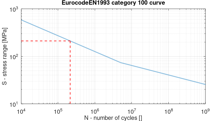
In this case, and assuming a Eurocode EN1993 S-N curve of category 100, it would take about
$$N=213{\ }000$$
cycles to reach failure. This means that this range will produce a damage of
$$d=1/N=4.68\cdot10^{-6}$$
Note: for half-cycles, the damage will be half.
Following the
Palmgren-Miner linear damage hypothesis, the damages produced by each new stress cycle are added together to obtain an
accumulated damage.
1.4 Fatigue life
The
Fatigue life is computed at each time step depending on how long the simulation has been running for. If the accumulated damage at time
$$t$$
is
$$d$$
, the fatigue life (in seconds) will simply be
$$f=t/d$$
.
This can be understood as follows: the fatigue life is the time it takes to reach failure, which by definition happens when
$$d=1$$
. Therefore (and assuming linear damage), if it took
$$t$$
seconds to reach an accumulated fatigue damage
$$d$$
, it will take
$$t/d$$
seconds to reach a damage of 1.
This is illustrated in the figure below:
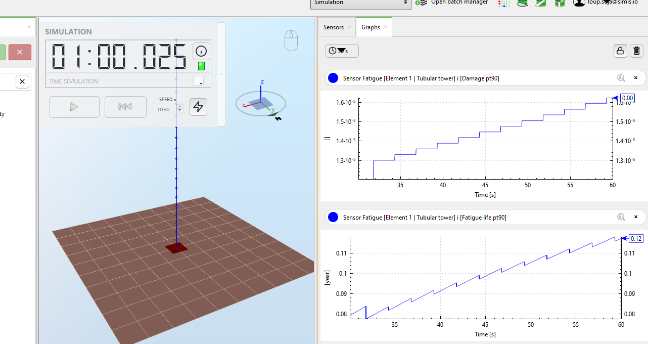
The accumulated damage after
$$t=60\text{ s}$$
is
$$d=1.6236\cdot10^{-5}$$
, therefore the fatigue life in years will be
$$F_L = t/(d\cdot3600\cdot24\cdot365)=0.117\text{ years}$$
Note: the fatigue damage is discontinuous (as seen in the figure above) because its value changes every time a new range is added, i.e. every time a new stress cycle has happened.
2 Fatigue life from histogram
This fatigue life estimation is done once the output file of the sensor is exported, or once the batch is finished (for batch simulations).
2.1 Retrieving stress time series
At the end of the batch, the
stress time series, which include the
SCFs defined by the user or pre-computed by Ashes, are retrieved from the results.
2.2 Performing the Rainflow counting algorithm
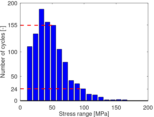
The stress time series goes through the
Rainflow counting algorithm, using the binning parameters provided in the fatigue tab of the
Preferences. The output of the counting is a load cycle histogram, that shows the number of cycles at a given stress range that happened during the simulation. The figure below is an example of such a histogram.
Note: the table containing this data can be found in the output file of the
Fatigue sensor (and currently not in the fatigue report)
2.3 Computing the damage
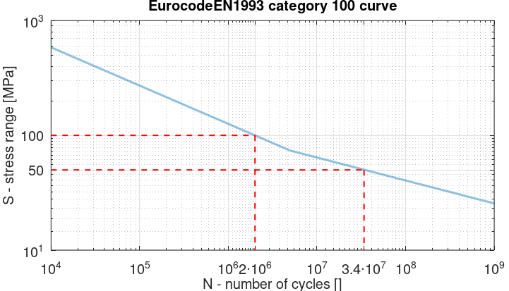
Once the histogram has been derived, the S-N curve is used to obtain the damage from each load cycle bin. Following the same procedure as in section 1.3 above, the figure below shows that the damage produced by one cycle of the 50 MPa bin is
$$d_{50}=1/3.4\cdot10^7=2.9\cdot10^{-8}$$
and the damage for the 100 MPa bin is
$$d_{100}=1/2\cdot10^6=5\cdot10^{-7}$$
Following the
Palmgren-Miner linear damage hypothesis, the damages produced by a given bin is equal to the damage of one cycle at the stress level of the bin multiplied by the number of cycles. For example, since there are 155 cycles at 50 MPa, the damage for the 50 MPa bin will be
$$155 \cdot d_{50}$$
The damages of each bin are then added together to obtain an accumulated damage.
2.4 Combining damages for the whole batch
At this point we have estimated the accumulated damage for one load case only. To obtain the combined damage for the batch, the damages from all load cases are multiplied by the probability of occurrence of that load case (which is set in the batch) and summed up.
The fatigue life is then obtained by following the same procedure as in section 1.4: if the combined damage for the load cases is
$$d$$
and the simulation duration is
$$t$$
, then te fatigue life in seconds is
$$t/d$$
.
The
Fatigue life from histogram estimate is the one that is provided in the Fatigue report produced after a batch run.
Note: the two estimates might be slightly different. This is because the ranges are binned in the
from histogram approach but not in the from Live approach. The bin definition can be found in the sensor output