Fatigue
1 Joints
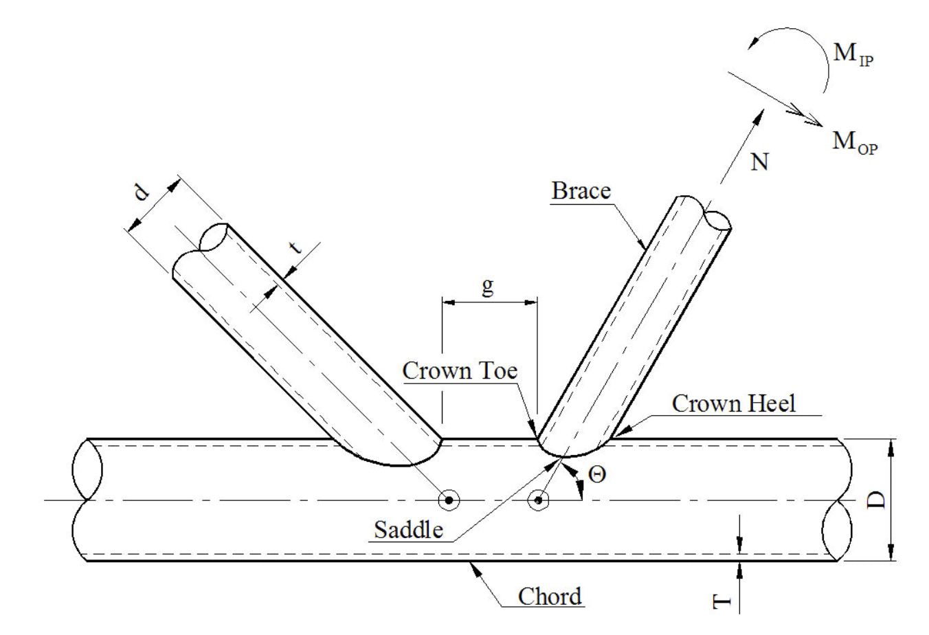
1.1 Geometrical definition of tubular joint
1.2 Joint definitions in support section text file
Joints
# Joint name   Chord elements  Brace elements
4-A    3&4    36&39
4-B    3&4    188&191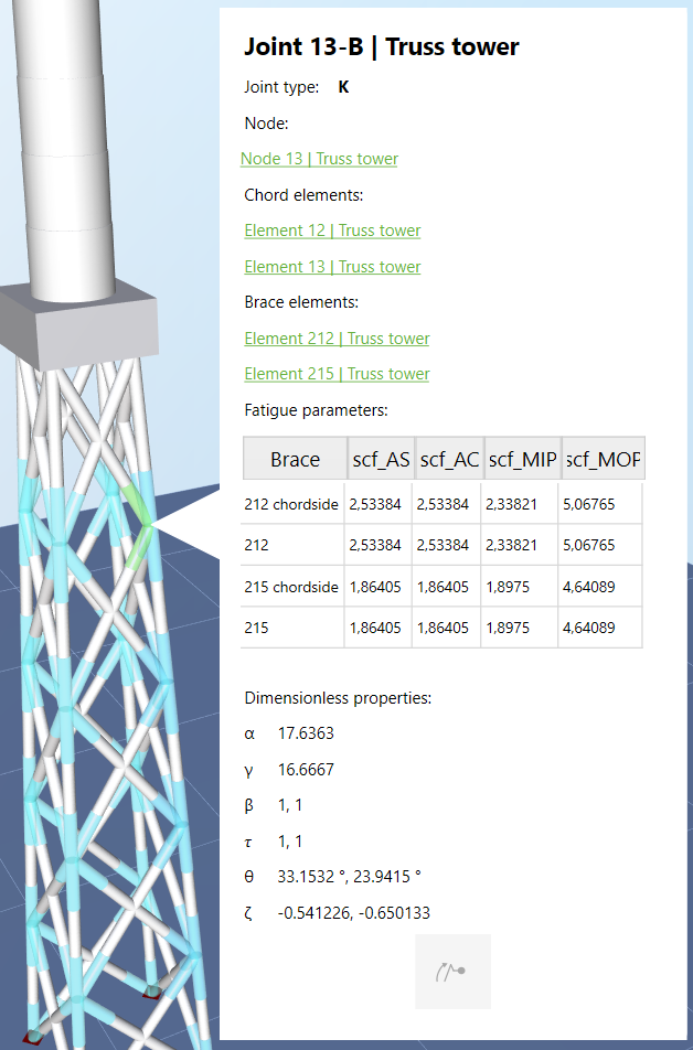
7-A 6&7 44&471.3 Selecting a Joint and viewing information
2 Stress calculations
2.1 Stress concentration factors (SCFs)
- $$\sigma_x$$: axial stress
- $$\sigma_{my}$$: bending stress from the moment about the y-axis. This stress arises from the in-plane bending moment, i.e. the bending moment that produces displacements of the braces within the joint plane.
- $$\sigma_{mz}$$: bending stress from the moment about the z-axis. This stress arises from the out-of-plane bending moment, i.e. the bending moment that produces displacements of the braces perpendicular to the joint plane.
- $$\text{SCF}_{\text{AC}}$$: axial stress concentration factor at crown
- $$\text{SCF}_{\text{AS}}$$: axial stress concentration factor at saddle
- $$\text{SCF}_{\text{MIP}}$$: in-plane bending stress concentration factor
- $$\text{SCF}_{\text{MOP}}$$: out-of-plane bending stress concentration factor
2.2 Hot spot stresses
| Hot spot | Field name in fatigue sensor |
| 1 | Stress pt0 |
| 2 | Stress pt45 |
| 3 | Stress pt90 |
| 4 | Stress pt135 |
| 5 | Stress pt180 |
| 6 | Stress pt225 |
| 7 | Stress pt270 |
| 8 | Stress pt315 |
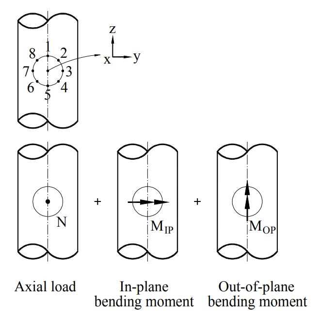
The normal stress at each of the 8 hot spots is calculated as a superposition of axial and bending stress contributions, each weighted by the appropriate stress concentration factor. The 8 equally-spaced points around the circular cross-section (at 0°, 45°, 90°, 135°, 180°, 225°, 270°, and 315°) account for combined axial and bending loads, where \(\sigma_x\) is the axial stress, \(\sigma_{\text{my}}\) is the in-plane bending stress, and \(\sigma_{\text{mz}}\) is the out-of-plane bending stress:
| (pt0°) | $$\sigma_1 = \text{SCF}_{\text{AC}}\, \sigma_x + \text{SCF}_{\text{MIP}}\, \sigma_{\text{my}}$$ |
| (pt45°) | $$\sigma_2 = \tfrac{1}{2}\!\left(\text{SCF}_{\text{AC}} + \text{SCF}_{\text{AS}}\right)\sigma_x + \tfrac{\sqrt{2}}{2}\,\text{SCF}_{\text{MIP}}\,\sigma_{\text{my}} - \tfrac{\sqrt{2}}{2}\,\text{SCF}_{\text{MOP}}\,\sigma_{\text{mz}}$$ |
| (pt90°) | $$\sigma_3 = \text{SCF}_{\text{AS}}\, \sigma_x - \text{SCF}_{\text{MOP}}\, \sigma_{\text{mz}}$$ |
| (pt135°) | $$\sigma_4 = \tfrac{1}{2}\!\left(\text{SCF}_{\text{AC}} + \text{SCF}_{\text{AS}}\right)\sigma_x - \tfrac{\sqrt{2}}{2}\,\text{SCF}_{\text{MIP}}\,\sigma_{\text{my}} - \tfrac{\sqrt{2}}{2}\,\text{SCF}_{\text{MOP}}\,\sigma_{\text{mz}}$$ |
| (pt180°) | $$\sigma_5 = \text{SCF}_{\text{AC}}\, \sigma_x - \text{SCF}_{\text{MIP}}\, \sigma_{\text{my}}$$ |
| (pt225°) | $$\sigma_6 = \tfrac{1}{2}\!\left(\text{SCF}_{\text{AC}} + \text{SCF}_{\text{AS}}\right)\sigma_x - \tfrac{\sqrt{2}}{2}\,\text{SCF}_{\text{MIP}}\,\sigma_{\text{my}} + \tfrac{\sqrt{2}}{2}\,\text{SCF}_{\text{MOP}}\,\sigma_{\text{mz}}$$ |
| (pt270°) | $$\sigma_7 = \text{SCF}_{\text{AS}}\, \sigma_x + \text{SCF}_{\text{MOP}}\, \sigma_{\text{mz}}$$ |
| (pt315°) | $$\sigma_8 = \tfrac{1}{2}\!\left(\text{SCF}_{\text{AC}} + \text{SCF}_{\text{AS}}\right)\sigma_x + \tfrac{\sqrt{2}}{2}\,\text{SCF}_{\text{MIP}}\,\sigma_{\text{my}} + \tfrac{\sqrt{2}}{2}\,\text{SCF}_{\text{MOP}}\,\sigma_{\text{mz}}$$ |
Note that at the crown points (0° and 180°), only \(\text{SCF}_{\text{AC}}\) and \(\text{SCF}_{\text{MIP}}\) contribute, while at the saddle points (90° and 270°), only \(\text{SCF}_{\text{AS}}\) and \(\text{SCF}_{\text{MOP}}\) apply. At the intermediate 45°-increment points, both axial SCFs contribute with equal weight and the bending terms are scaled by \(\tfrac{\sqrt{2}}{2} \approx 0.707\).
Location of pt0: crown heel or crown toe
The location of pt0 in Ashes is always at either the crown heel or the crown toe, depending on the order of the nodes in which the brace element was defined in the text file:
- If node 1 in the element definition is the joint node (i.e. the node at the intersection with the chord) and node 2 is the outer node, then pt0 will be at the crown heel and pt180 will be at the crown toe, as defined in DNV-RP-C203.
- If node 1 is the outer node and node 2 is the joint node, the assignment is reversed: pt0 will be at the crown toe and pt180 will be at the crown heel.
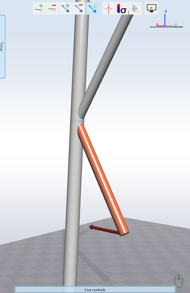
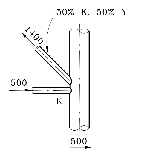
As defined in DNV-RP-C203, compression produces a negative stress. In the figure below, the applied load produces a compressive in-plane bending moment at the crown heel (resulting in a negative stress at the corresponding stress point) and a tensile in-plane bending moment at the crown toe. This sign convention can be used to verify that the stress points are correctly defined in the model.
2.3 Classification of joints
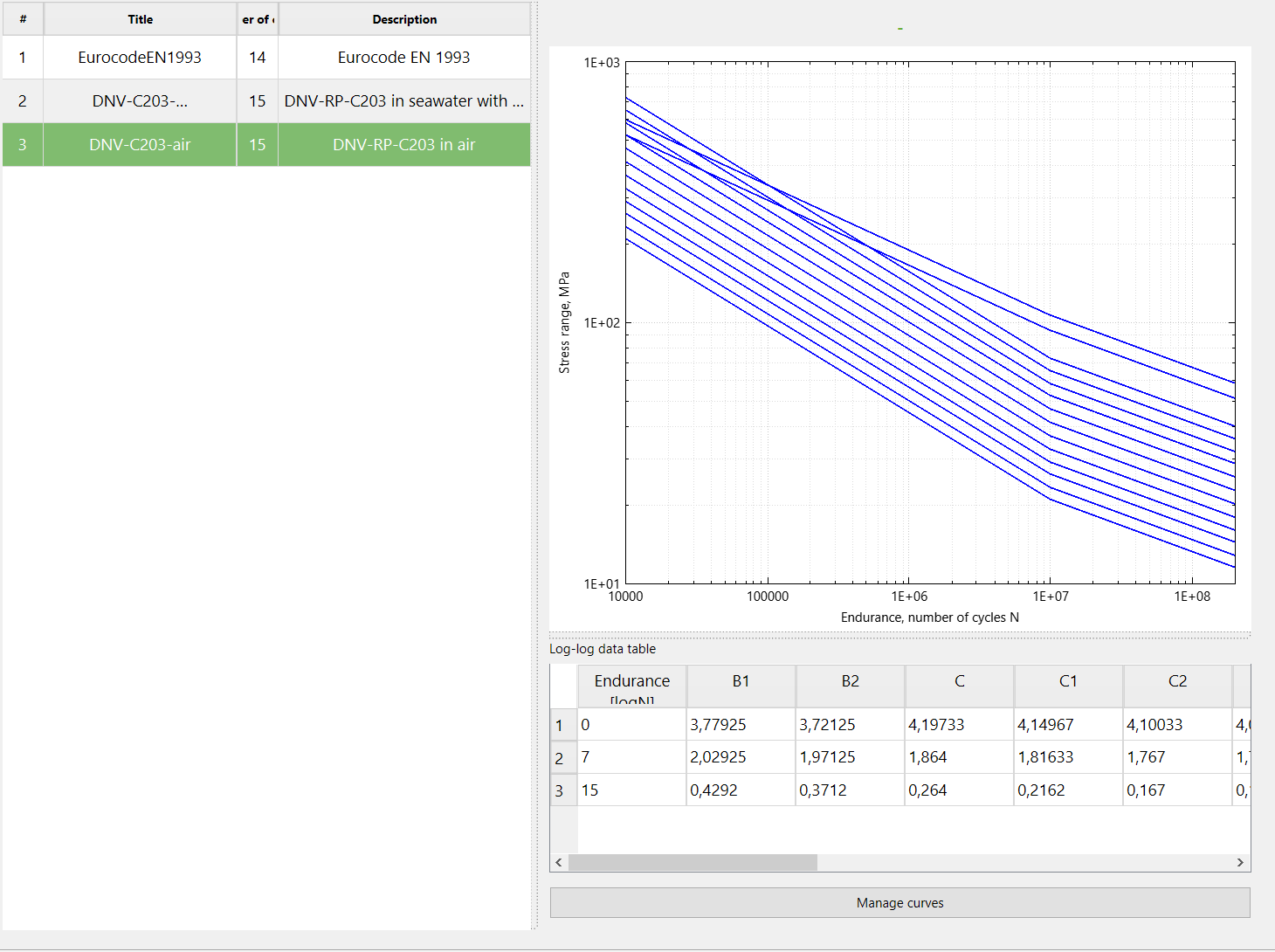
3 S-N curves
3.1 Assigning S-N curves to joints and sensors
4 Workflow
4.1 Relevant settings and parameters
4.2 Workflow summary
- Define Joints. Specify each joint to be included in fatigue computations in the Joints section of the support section file, then import it (this is only required if you perform a fatigue analysis on a truss tower).
-
Add sensors. Right-click each joint and click the Add sensor button. For joints, this will
produce two sensors for each brace, one for stresses chordside and one for braceside. If you want to add a sensor for every
joint, click
 in the Sensors
window and choose Add fatigue sensors to all Joints.
in the Sensors
window and choose Add fatigue sensors to all Joints.
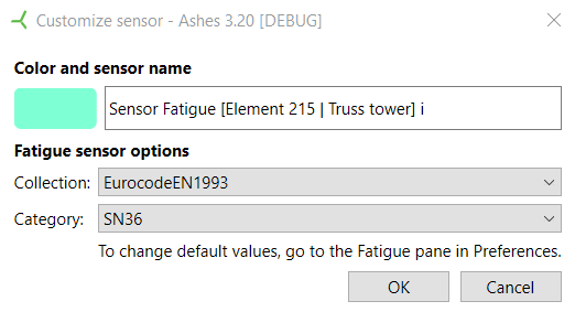
- Assign S-N curve and category. Each sensor will be assigned default S-N settings when they are added. To change these settings, right-click the sensor and choose Options. Default S-N settings can also be assigned per joint in the Joints section of the support section file.
- Run simulation(s). Run your simulations, either in Time simulation or in Batch. The fatigue sensors will collect stress ranges for each hot spot during simulation.
-
View report. If you run in Time simulation, you can generate the fatigue report by clicking
 in the Sensors window and checking
the Generate fatigue report...option. If you run in batch, there will be report PDF file called
Jointssummary.pdf placed in the results folder.
in the Sensors window and checking
the Generate fatigue report...option. If you run in batch, there will be report PDF file called
Jointssummary.pdf placed in the results folder.