Note: this is only valid because the rotational speed is zero, which implies that there is no induced velocities
One airfoil blade fixed
1 Test description
This test uses a simple blade with few aerodynamical blade stations in steady conditions and compares the aerodynamical loads computed by Ashes to an analytical solution.
The following load cases are tested
- Stiff blade
- Two-element blade
- Three-element blade
- 20-element blade
2 Model
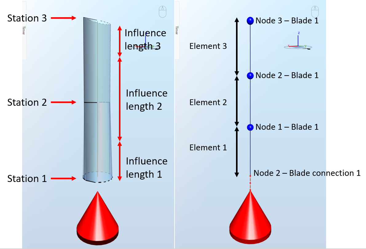
The model used for this test is shown in the figure below:

The chordlength accross the blade is
$$c = 1\text{ m}$$
, the blade length is
$$L = 5\text{ m}$$
and the hub radius is
$$r_h = 0.5\text{ m}$$
.
The rotor is fixed, the blade is therefore not rotating. For the models that do not use the
Stiff rotor approximation, the blade and the hub conections are infinitely stiff, therefore there are no deflections.
The blade used for this model has three
Blade aerodynamical station. The innermost station is at the root and has a cylindrical airfoil with
no drag and no lift. This station will therefore not produce any aerodynamic loads.
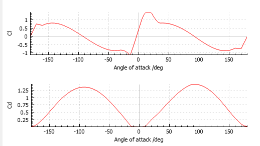
The two other blade aerodynamical stations have the
NACA64-618 airfoil, which polar can be exported from Ashes and are shown in the figure below:
The table below gives a summary of the relevant blade characteristics:
| Blade aerodynamical station | Distance to blade root | Influence length | Airfoil |
| 1 |
$$r_1 = 0$$
|
$$L_{I1} = 1.25\text{ m}$$
|
Cylinder with no lift and drag |
| 2 |
$$r_2 = 2.5\text{ m}$$
|
$$L_{I2} = 2.5\text{ m}$$
|
NACA64-618 |
| 3 |
$$r_3 = 5\text{ m}$$
|
$$L_{I3}=1.25\text{ m}$$
|
NACA64-618 |
The air density is
$$\rho = 1.225\text{ kg}\cdot{m}^{-3}$$
. No gravity forces are applied, and tip and hub corrections are set to 0.3 Analytical solution
3.1 For stiff blades
The wind speed speed is denoted
$$V$$
. For the current analysis we use
$$V = 10\text{ m}\cdot\text{s}^{-1}$$
Since there is no rotational velocity, the angle of attack at all blade aerodynamical stations is 90 degrees. For the two outermost blade aerodynamical stations, this gives a lift and drag coefficient of
$$C_L = 0.053$$
and
$$C_D = 1.4565$$
(the innermost blade aerodynamical blade station experiences no lift or drag, and is therefore not considered in the rest of the analysis).
For blade aerodynamical station
$$i$$
, the distributed lift and srag forces are, respectively:
$$F_{L,i}=\frac{1}{2}\rho c C_L V^2$$
and
$$F_{D,i}=\frac{1}{2}\rho c C_D V^2$$
The
aerodynamic thrust
for the whole rotor is thus
$$F_T = \sum_{i=2}^3F_{D,i}\cdot L_{Ii}=334.5\text{ N}$$
and the
aerodynamic torque for the whole rotor is
$$T=\sum_{i=2}^3 F_{L,i}\cdot L_{Ii}\cdot (r_i+r_h)=46.67\text{ Nm}$$
. These two output can be found in the
Rotor sensor.
The next three output are part of the
Blade [Time] sensor sensor. The
root force
is the sum of the drag and the lift forces from both stations, which can be expressed as
$$F_r = \sum_{i=2}^3\sqrt{(F_{D,i}\cdot L_{I,i})^2+(F_{L,i}\cdot L_{I,i})^2}=334.8\text{ N}$$
. The
in-plane bending moment is
$$M_{ip}=\sum_{i=2}^3 F_{L,i}\cdot L_{Ii}\cdot r_i=40.58\text{ Nm}$$
and the
out-of-plane bending moment is
$$M_{oop}=\sum_{i=2}^3F_{D,i}\cdot L_{Ii}\cdot r_i=1115\text{ Nm}$$
3.2 For flexible blades
Flexible blades, as opposed to stiff blades, are modelled structurally by dividing the blade into a number of finite elements, each with its own structural properties (which can be different for each element or the same accross the blade span, as is the case in this model). In the present test, flexible blades are modelled with elements that have a very large stiffness, which means that they will experience no deflection.
Because Flexible blades are divided into structural elements, the aerodynamic loads have to be lumped and applied to the nodes at both ends of the element. The lumping is done as follows: if part of an element lies within the
Influence length of an
Blade aerodynamical station, its nodes will experience aerodynamic loads. Each of the two loads (one on each node) will be equal to the linear aerodynamic loads multiplied the portion of the element that lies within the Influence length divided by two.
Below we show several examples of how the derivation is carried out for the present test.
3.2.1 Two-element blade
This blades has two elements, of half a blade length each.
A two-element blade will have three structural nodes, each located at a Blade aerodynamical station. The Influence length of each Blade aerodynamical station will vary depending on its position along the blade (a detailed explanation of how the influence length is obtained can be found in the
Influence length document). This is illustrated in the figure below:
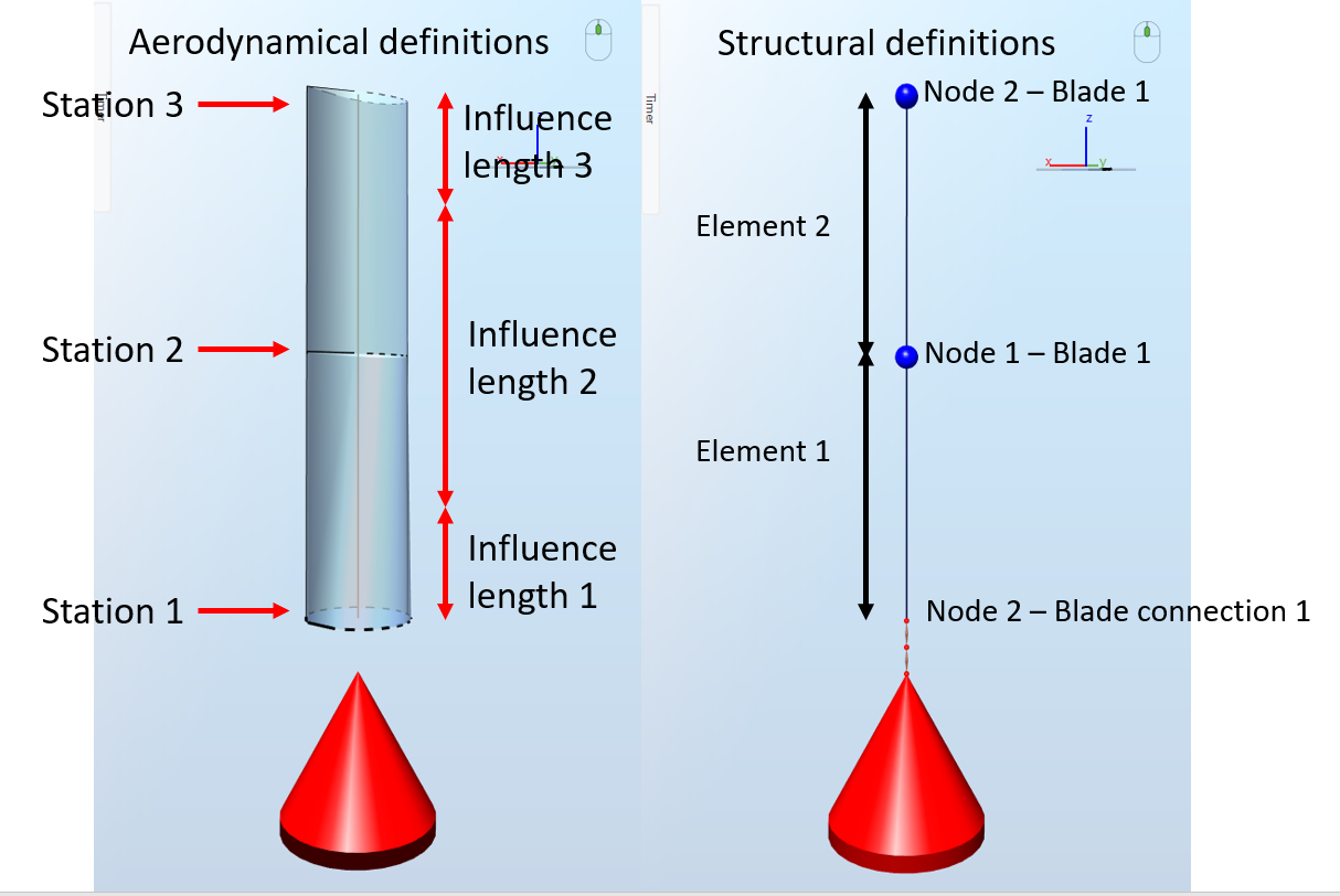
Note: there are two more nodes in this model, that belong to the Blade connection. These have been hidden in the picture of the left
To exemplify how the loads apply on each node, we first focus on the drag force and how it contributes to the Aerodynamic thrust.
As explained above, the drag force from station 3 will be
$$F_{D,3}\cdot L_{i,3}=111.5\text{ N}$$
. The influence length of this station is entirely within Element 2, so this load will only be applied to Element 2.
The drag force from station 2 will be
$$F_{D,2}\cdot L_{i,2}=223.0\text{ N}$$
Half on its influence length is on Element 2 and the other half on Element 1, which means that half of this load will be applied on Element 2 and the other half on Element 1. This means that Element 2 will experience a total load (from two stations) of
$$111.5+223.0/2=223.0\text{ N}$$
In Ashes, the loads experienced by an element are divided by two and lumped to its nodes. This means that, from Element 2 (namely Node 1 and Node 2 from Blade 1) will experience a load (more precisely, a BEM nodal load) in the direction of the drag of
$$111.5\text{ N}$$
. This is illustrated inthe figure below: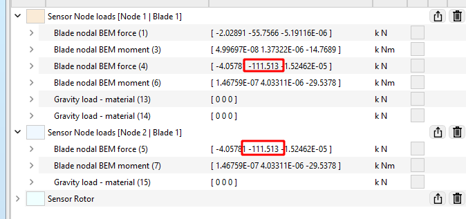
Note: in the above picture, not all possilbe fields from the
Loads on node sensor are displayed. You can customise which fields are displayed in the
Customise sensor fields document.
Similarly, since half of the influence length of station 2 is on Element 1, half of the drag load from station 2 will be applied to Element 1. This will be the only drag load applied to Element 1 since station 1 does not experience aerodynamic loads (because its lift and drag coefficients are both 0), so it will have a value of
$$F_{D,2}\cdot (L_{i,2}/2)=111.5\text{ N}$$
. The load on Element 1 will be split into two equal components applied to both of its nodes, of value
$$55.75\text{ N}$$
. This is illustrated in the figure below: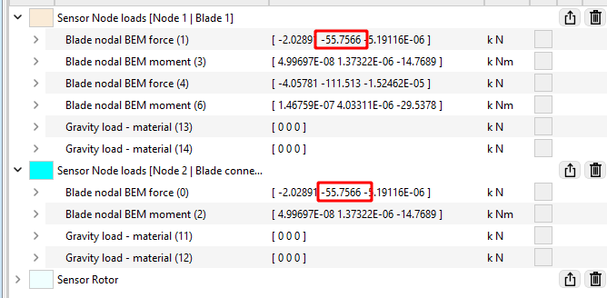
The sum of all the BEM forces in the drag directions amounts to
$$334.5\text{ N}$$
, which is the value of the thrust force on the rotor
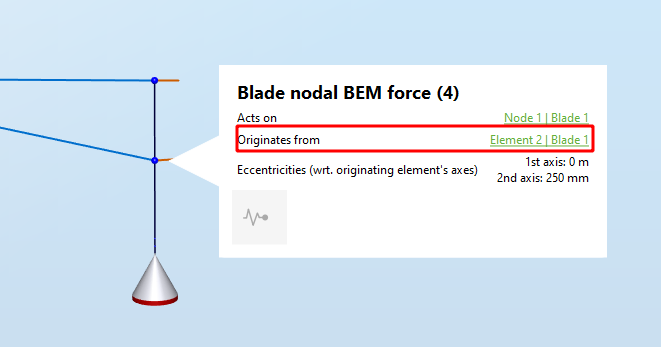
It is important to note that the way the aerodynamical loads are lumped onto structural nodes has implications on the bending moments at the blade root. For example, part of the drag from station 2 is applied to the node at the root of the blade (or more precisely,
Blade nodal BEM force (0) is applied on
Node 2 - Blade connection 1). This means that it will not contribute to the Out-of-plane bending moment. If we use the notation
$$BEM_{i,y}$$
to mean the y-component Blade nodal force (i) (i.e. the component in the drag direction) and by noticing that both elements have a length
$$E_L = 2.5\text{ m}$$
, we find that the Out-of plane bending moment will be
$$M_{oop,f}=BEM_{1,y}\cdot E_L+BEM_{4,y}\cdot E_L+BEM_{5,y}\cdot 2E_L=976\text{ Nm}$$
As expected , this value is lower than the Out-of-plane bendig moment with stiff blades, since part of the aerodynamic loads are applied at the root.
This lumping will also influence the aerodynamic torque. By following the same procedure as above including the hub radius, we obtain an aerodynamic torque in the Flexible blades case of
$$T = BEM_{0,x}\cdot r_h+BEM_{1,x}\cdot (E_L+r_h)+BEM_{4,x}\cdot (E_L+r_h)+BEM_{5,x}\cdot (2E_L+r_h)=41.59\text{ Nm}$$
Again, this is lower than with Stiff blade case.
Note: to simplify the equations, we have ommitted the negative signs in front of the components of the Blade nodal forces. A detailed explanation of the signs for the bending moments can be found in the
Out-of-plane and
In-plane documents. The aerodynamic torque is positive when it spins the rotor clockwise.
3.2.2 Three-element blade
We now reproduce the derivation explained in the previous paragraph for a blade divided into three elements, shown in the image below:
- for Station 3,
$$F_{D,3}\cdot L_{I,3}=111.5\text{ N}$$
- for Station 2,
$$F_{D,2}\cdot L_{D,2} = 223.0\text{ N}$$
- for Station 3,
$$0\text{ N}$$
Element 3 covers the whole Influence length 3 and one sixth of Influence length 2, therefore it will experience a drag force of
$$111.5+223.0/6=148.7\text{ N}$$
. This force is then split in two and the resulting force of
$$74.33\text{ N}$$
is applied to both nodes of element 3 (namely Node 2 and Node 3 on Blade 1).
Element 2 covers two thirds of Influence lenght 2, therefore it will experience a drag force of
$$223\cdot2/3=148.7\text{ N}$$
. Its nodes (namely Node 2 and Node 1 from Blade 1) will thus experience a force of
$$74.33\text{ N}$$
.
Element 1 covers one sixth of influence length 2 and the whole Influence length 1, but the latter does not produce any aerodynamic load. It will therefore experience a drag force of
$$223/6 = 31.27\text{ N}$$
and its nodes (namely Node 1 from blade 1 and Node 2 from Blade connection) will experience a force of
$$18.59\text{ N} $$
.
If we now calculate the out-of-plane bending moment as we did for the two-element blade case, we find that
$$M_{oop,3}=1022\text{ Nm}$$
.
Similarly, the aerodynamic torque is now
$$T=42.95\text{ Nm}$$
.
These values are again lower than the case of stiff blades, but are larger than the case with two elements. This is expected since the load applied at the root of the blade (Node 2 of Blade connection) is lower than in the two-element case.
3.2.3 Analytical solution
If we consider the case of a cantilever beam with a partial distributed load, we can find the analytical solution for the bending moment at the root of the beam. This case is illustrated in the figure below:
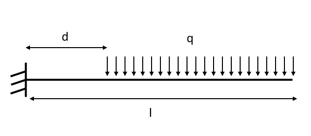
The bending moment at the root of the beam is
Applying this formula to the blade bending moments and aerodynamic torque, we find
$$M = q\frac{\left(l^2-d^2\right)}{2}$$
Applying this formula to the blade bending moments and aerodynamic torque, we find
$$M_{oop,an}=F_{D}\frac{L^2-L_{I,1}^2}{2}=1045\text{ Nm}$$
$$M_{ip,an}=F_{L}\frac{L^2-L_{I,1}^2}{2}=38.04\text{ Nm}$$
$$T_{an}=F_{L}\frac{(L+r_h)^2-(L_{I,1}+r_h)^2}{2}=44.13\text{ Nm}$$
A blade with an inifinite number of elements should produce these results. In practice, we expect that 20 elements should be enough to get with 0.05% of the analytical solution.
3.3 Summary of expected results
The following table sums up the results expected in Ashes, as calculated above:
| Test name |
Aerodynamic thrust
$$[\text{N}]$$
|
Aerodynamic torque
$$[\text{Nm}]$$
|
Root force
$$[\text{N}]$$
|
In plane bending moment
$$[\text{Nm}]$$
|
Out of plane bending moment
$$[\text{Nm}]$$
|
| Stiff blade | 334.5 | 46.67 | 334.8 | 40.58 | 1115 |
| two-element blade | 334.5 | 41.59 | 334.8 | 33.50 | 975.4 |
| three-element blade | 334.5 | 43.28 | 334.8 | 37.20 | 1022 |
| 20-element blade | 334.5 | 44.13 | 334.8 | 38.04 | 1045 |
4 Results
A simulation of ten seconds is run. The test is considered passed if the last two seconds of the results produced by Ashes lie within 0.05% of the expected solution.
The report with the results can be found here: