Irregular linear waves
Irregular waves are simulated by a linear superposition of
Regular waves, i.e. sine wave components. The velocity potential that describes irregilar waves can then be obtained by summing up the individual velocity potentials of the regular waves, such as
$$\Phi = \sum_{i=1}^N\frac{gA_{i}}{\omega_i}\frac{\cosh\left[k_i(z+h)\right]}{\cosh(k_ih)}\cos(\omega_i t +k_ix - \epsilon_i)$$
where
$$i$$
denotes the i
th component of the irregular waves. The phase angles
$$\epsilon_i$$
are randomly selected within a uniform distribution between
$$-\pi$$
and
$$\pi$$
. The number of components is determined by
$$N$$
and can be adjusted with the
N parameter in the
Irregular waves-single spectrum part. The irregular wave elevation is given by
$$\zeta = \sum_{i=1}^NA_{i}\sin(\omega_it+k_ix - \epsilon_i)$$
The amplitude of each component is given by a wave spectrum
$$S(\omega)$$
such that
$$\frac{1}{2}A_{i}^2 = S(\omega_i)d\omega_i$$
where
$$d\omega_i=\omega_{i+1}-\omega_i$$
. Different spectra can be used to represent irregular seas. In Ashes, the
default spectrum is the JONSWAP spectrum (see
Hasselmann et al. (1973)
), which is a modification of the Pierson-Moskowitz spectrum. The power spectral density for a Pierson-Moskowitz spectrum
depending on the wave circular frequency ω is given by the following formulae (see
DNV-GL (2017a)
):
$$S_{PM} = {5 \over 16} \cdot H_S^2 \cdot \omega_P^4 \cdot \omega^{-5} \cdot \exp \left(- {5 \over 4} \left( \omega \over \omega_P \right)^{-4}\right) $$
Where
H
S
is the significant wave height [m]
ω
P
is the spectral peak angular frequency, given by ω
P
= (2π)/(T
P) [rad⋅s − 1]
T
P
is the spectral peak period [s]
The power spectral density for a JONSWAP spectrum is obtained from the Pierson-Moskowitz spectrum following
$$B = exp \left(-0.5 \left( {\omega - \omega_P} \over {\sigma \cdot \omega_P} \right)^2 \right)$$
$$S_J(\omega) = A_\gamma \cdot S_{PM}(\omega) \cdot \gamma^B$$
Where
A
γ
= 1 − 0.287ln(γ)
γ is the non-dimensional peak shape parameter [-] (also called peakedness or gamma factor)
σ is the spectral width parameter [-] given by
σ = 0.07 for ω ≤ ω
P
σ = 0.09 for ω > ω
P
It can be seen from the previous equations that a Pierson-Moslowitz spectrum can be chosen in Ashes by selecting γ = 1.
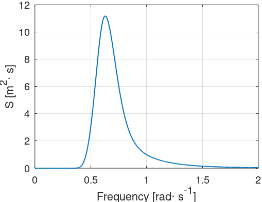
The figure below illustrates the JONSWAP spectrum for
$$H_S = 6\text{ m}$$
,
$$T_P = 10\text{ s}$$
and
$$\gamma = 3.3$$
.
It is common to represent different realizations of a spectrum, i.e. computations of the wave elevation that have the same significant wave height
$$H_S$$
, spectral peak period
$$T_P$$
and peak shape
$$\gamma$$
but that produce different wave elevation time series. This is achieved by changing the seed with which the phase anlges
$$\epsilon_i$$
are randomly computed. This is done using the
Seed parameter in the
Irregular waves-single spectrum part. By keeping a constant seed, the same realization of the irregular seas will be carried out, thus producing the same wave elevation time series. In addition, there are two options for generating wave components that can be selected from the
Simulation scheme
parameter of the
Irregular waves-single spectrum part:
-
Equal frequency
The amplitude of each wave component will be computed based on the selected wave spectrum with a constant
$$d\omega_i$$
.
-
Equal energy
Each wave component represents the same energy (i.e. the same area of the wave spectrum).
1
Max and Min frequencies
There is a range of frequency outside of which the spectral density can be neglected. The sinusoidal components that have their frequencies outside that range will not have a significant influence on the wave kinematics, it is therefore common to truncate the spectrum at those frequencies.
The width of this range is determined by the
Error estimate
parameter in the
Irregular waves-single spectrum part. Here we explain the procedure assuming an error estimate
$$\epsilon = 0.01 = 1\%$$
and a JONSWAP spectrum
$$S(\omega)$$
with
$$H_S = 6\text{ m}$$
,
$$T_P = 10\text{ s}$$
and
$$\gamma = 3.3$$
.
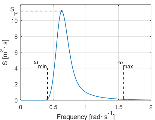
First we estimate the spectral density around the spectral peak period
$$S_P = S(2\pi/T_P)$$
.
We then find the two frequencies
$$\omega_{min}$$
and
$$\omega_{max}$$
for which the spectral density is
$$S(\omega_{min}) = S(\omega_{max})=\epsilon\cdot S_P$$
.
The frequencies that are taken into account when computing the wave kinematics are then
$$\omega \in [\omega_{min}\text{ } \omega_{max}]$$
The figure below illustrates the frequency range and the maximum spectral density.
2 Simulation scheme
When simulating irregular waves in Ashes, the
Simulation scheme parameter allows you to chose between
Equal frequency or
Equal energy. These two options relate to the discretisation of the frequency range and define how the components of the spectrum are obtained. Both methods are explained below.
2.1
Equal frequency
When this option is selected, the frequency step is kept constant and is equal to
$$d\omega =\frac{\omega_{max}-\omega_{min}}{N}$$
where
$$N$$
is the number of components.
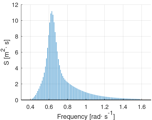
The figure below illustrates the JONSWAP spectrum used previously with the
Equal frequency option and
$$N = 100$$
Note: If all the discretisation frequencies are a multiple of
$$dw$$
, the wave elevation will repeat irself after an amount of time
$$T_{rep}=2\pi/d\omega$$
. With the example above, the repetition time is around 537 s.
In addition, the
Equal frequency method might result in a coarse discretisation of frequencies around the peak of the spectrum.
Both this problems can be solved by increasing the number of components
$$N$$
. The standard
DNV-GL (2017a) recommends using
$$N = 1000$$
. However, such a large number of components requires more operations to be performed and results in the simulation running too slow for practical uses.
It is therefore recommended to use the
Equal energy scheme.
When chosing the
Equal frequency scheme, the equation
$$\frac{1}{2}A_{i}^2 = S(\omega_i)d\omega_i$$
then becomes
$$\frac{1}{2}A_{i}^2 = S(\omega_i)d\omega$$
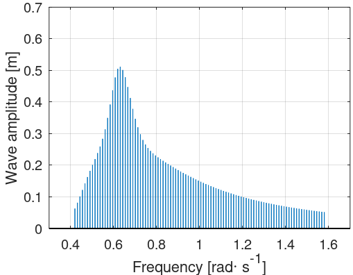
The amplitude of each component can thus be obtained, and the amplitude spectrum can be plotted, as shown in the figure below:
Note: in order to extend the range of frequencies considered, the parameter
Error estimate can be lowered (see section
Max and Min frequencies)
2.2
Equal energy wave components
When this option is selected, the frequency step for each component
$$d\omega_i$$
is selected so that each component in the spectrum has the same energy content. Since the energy is equal to the area under the spectrum, this method is sometimes refered to as
Equal Area. This is done as follows:
-
the total energy content in the spectrum between
$$\omega_{min}$$
and
$$\omega_{max}$$
, hereafter refered to as
$$E_{tot}$$
, is obtained by geometrical integration of the area under the spectrum
-
the energy for each component is obtained by dividing the total energy by the number of components:
$$dE = E_{tot}/N$$
-
the discretisation frequencies are chosen so that
$$(\omega_{i+1}-\omega_i)\cdot S\left(\frac{\omega_i +\omega_{i+1}}{2}\right)=dE$$
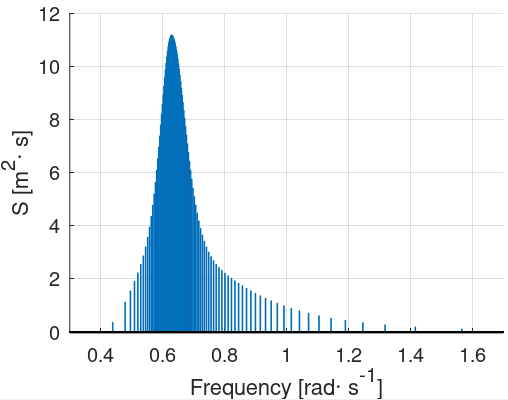
This results in a non-constant frequency step accross the spectrum. The figure below illustrates the JONSWAP spectrum used previously with the
Equal energy
scheme and
$$N=100$$
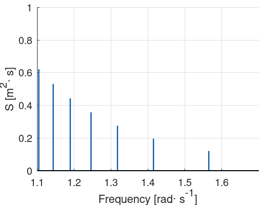
Note how in the figure above, the last components cover a wide frequency range compared to the other components. This means that there will be comparatively fewer components modeling the higher frequencies of the spectrum, which can be a problem when simulating the response of certain structures. The figure below offers a zoom of the tail of the previous spectrum.
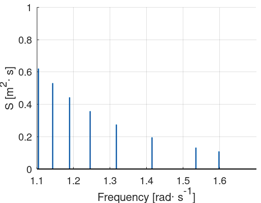
In order to solve this issue, it is possible to further divide each of these frequency bins into smaller bins. The parameter
Frequency delta limit
allows you to set a maximum frequency width for each component as a product of the average difference between two consecutive frequencies. The figure below illustrates a case where the
Frequency delta limit is set to 10. In the previous figure, the difference between the frequencies of the last and the prelast components was more than 10 times the average difference, therefore an additional component was added.
Note:
this implies that you can end up with more than
$$N$$
components, and that the extra components will not have the same energy as the rest.
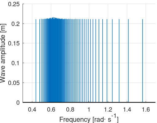
Another effect of using the
Equal energy scheme is that all components will have the same amplitude This is because the energy of a component is proportional to its amplitude square, through
$$dE=0.5\rho g A^2$$
. The image below shows the amplitude spectrum.
With the
Equal energy scheme, the repetition time becomes much larger than the typical simulation times for offshore wind turbines. In practice, it is safe to consider that the simulation does not repeat.