Dynamic stall test
1 Test description
This test verifies that the results produced by Ashes are the same as the ones presented in the dynamic stall section in
Hansen (2008d). The implementation of the dynamic stall model in Ashes is presented in the
Unsteady BEM section of the theory manual.
2 Model
The model has been generated to match the data from
Hansen (2008d).
No numerical data in given for the polars used, only the graph in figure 9.9 is provided. The polars used in Ashes have been extracted from that figure and added to the airfoil
Dynamic stall test, which can be found in the
Airfoil database. Note that only data from 0 to 18 degrees is provided, so we have added arbitrary (but realistic) values to fill the -180 to 180 degrees range.
The rotor is stationary (i.e. not rotating) so that no induced velocity is created when applying the BEM theory. The incoming wind speed is constant at
$$10\text{ m}\cdot\text{s}^{-1}$$
and the incoming wind angle varies sinusoidally such as
$$\alpha = 15+2\sin{(12.57\cdot t)}$$
, where
$$t$$
is the temporal coordinate, as specified in
Hansen (2008d).
The blade has a chord length of 0.2 m, in order to get a time constant
$$\tau=0.08\text{ s}$$
(see
Unsteady BEM) as specified in
Hansen (2008d).3 Benchmark solution
Following the implementation of
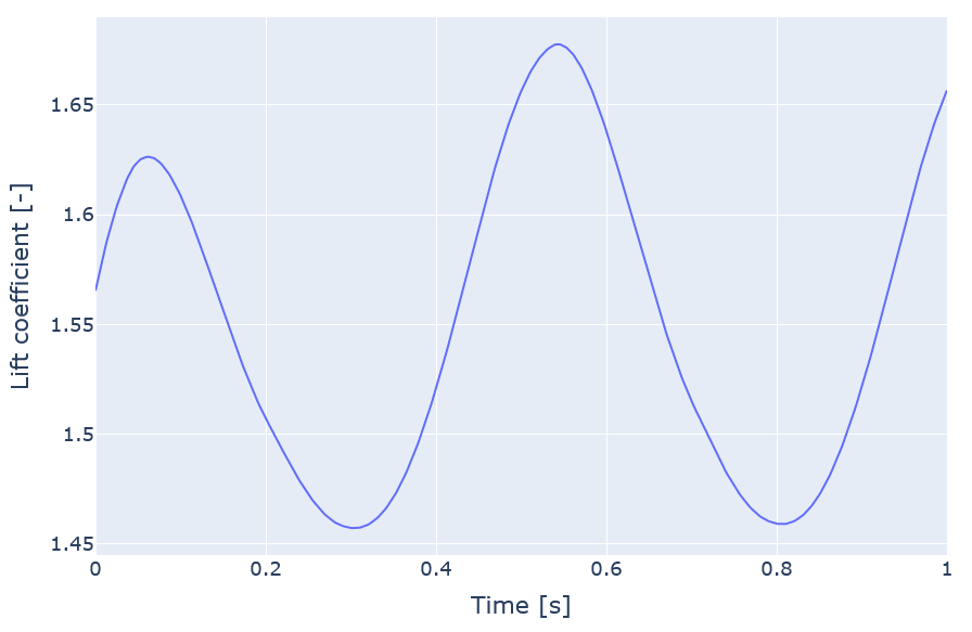
Hansen (2008d), the variation of the lift coefficient over one second will be as shown in the following figure:
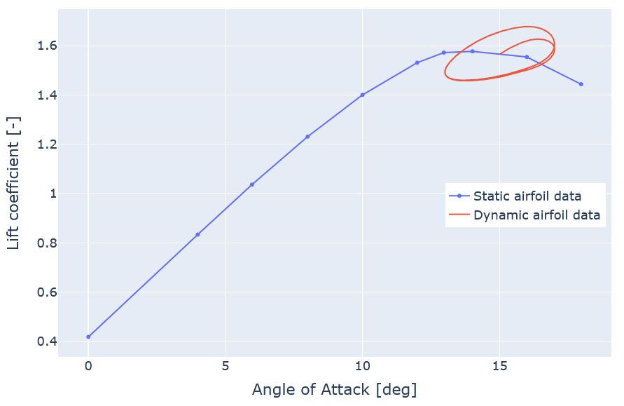
When plotted on the polar, the hysteresis due to the dynamic stall model becomes visible:
4 Results
The test is considered passed if the last 20% of the results from Ashes are within 1% of the benchmark solution. Note that Ashes use a different initial condition than
Hansen (2008d), it is therefore not expected that the results will match during the transient period.
The report can be downloaded from the following link: