- The BEM theory uses the projection of the wind velocity in the blade station plane, which is here simply refered to as wind velocity.
- The wind velocity is not in general perpendicular to the rotational velocity, i.e. it can have a component in the rotational velocity. For simplicity, in this section, any such component is added to the rotational velocity.
Steady BEM
The basic steady BEM algorithm makes an initial assumption on the value of the induced velocity. By means of
blade element theory, this induced velocity is used to compute the lift and drag forces on a blade element. The
conservation of momentum
is then applied with these aerodynamic loads to calculate a new induced velocity. This new induced velocity is then compared to the initial assumption. If the two don't match within a certain margin, the new induced velocity is used as an input for the blade element theory and the process is repeated, until convergence is achieved. Two important assumptions of the BEM theory are
- Blade elements behave independently of each other.
- An infinite number of blades is assumed. This is corrected for by adding the Prandlt correction (see Hansen (2008d))
In the following we describe the algorithm applied on one blade element. The aerodynamic loads and induced velocities are computed within the
Blade aerodynamical station plane. This plane, in which the
Velocity triangle is shown, is perpendicular to the axis formed by the two nodes composing the blade element and lies at half the distance between the two. This implies that the Blade aerodynamical station plane follows the displacements of the blade element due to the elasticity of the blade. The follwing picture is drawn in the blade aerodynamical station plane:

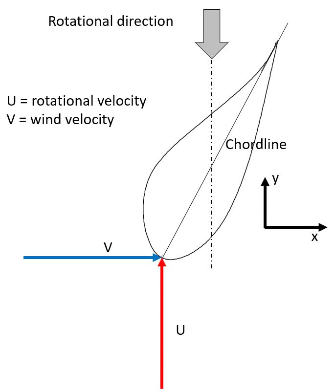
We define the vectors
x
and
y
as unit vectors in the blade aerodynamical station plane such that
y is in the rotational direction and
x is perpendicular to
y. In the present example, the blade station moves in the rotational direction, which produces a rotational velocity felt by the blade station in the opposite direction.
Notes:
The steps followed in the steady BEM algorithm are listed and described below:
1 Initial estimation of the induced velocity
An initial guess is made on the induced velocity:
- the projection of the induced velocity in the x-direction, called axial induced velocity and noted V i, is assumed to be 0.33 times the wind velocity
- the projection of the induced velocity in the y-direction, called tangential induced velocity and noted U i, is assumed to be 0.
it is common to define the
axial induction factor
a and the
tangential induction factors
a' as
$$a=\frac{|V_i|}{|V|}$$
,
$$a'=\frac{|U_i|}{|U|}$$
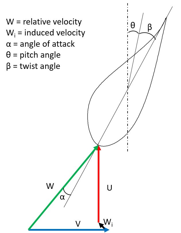
2 Compute the angle of attack
At this stage, the induced velocity (noted
W
i) is taken from the previous iteration. The angle of attack (noted
$$\alpha$$
) is the angle between the relative velocity and the chordline. The relative velocity (noted
W) is the sum of the wind, rotational and induced velocities. The angle of attack is then obtained with the following equation
$$\alpha = \tan^{-1}\left(\frac{V(1-a)}{U(1+a')}\right)-\beta-\theta$$
This is illustrated in the figure below
3 Look up the aerodynamic coefficients
Based on the angle of attack, the polars of the airfoil defined in the
Airfoil polar file
are looked up to obtain the lift, drag and moment coefficients
$$C_L, C_D$$
and
$$C_m$$
. If, for the considered airfoil, different polars are given at different Reynolds numbers, a
local Reynolds number is computed following
$$Re = \frac{|W|\cdot C}{\nu}$$
where
$$C$$
is the chordlength (or the diameter for circular elements) and
$$\nu$$
is the kinematic viscosity of the air (set in the
Atmosphere
parameter). If the local Reynolds number thus calculated does not correspond to a Reynolds number for which a polar is given, the aerodynamic coefficients will be interpolated between the two closest polars. A linear or a logarithmic interpolation scheme can be chosen in the
Aerodynamics tab of the
Analysis parameters.
If the angle of attack does not correspond to a value given in the polars, a linear interpolation is performed between the two closest given values.
4 Compute aerodynamic forces
Once the aerodynamic coefficients have been established, the lift and drag forces are calculated with the following equations:
$$F_L=C_L\frac{1}{2}\rho|W|^2C\cdot L$$
$$F_D=C_D\frac{1}{2}\rho|W|^2C\cdot L$$
where
$$L$$
is the
Influence length of the blade aerodynamical station and
$$\rho$$
is the density of the air (that can be changed in the
Atmosphere
parameter).
For a given blade aerodynamical station, the
Influence length is defined as the distace between the middle point between the current blade station and the next blade station and the middle point between the current blade station and the next blade station, as illustrated in the image below
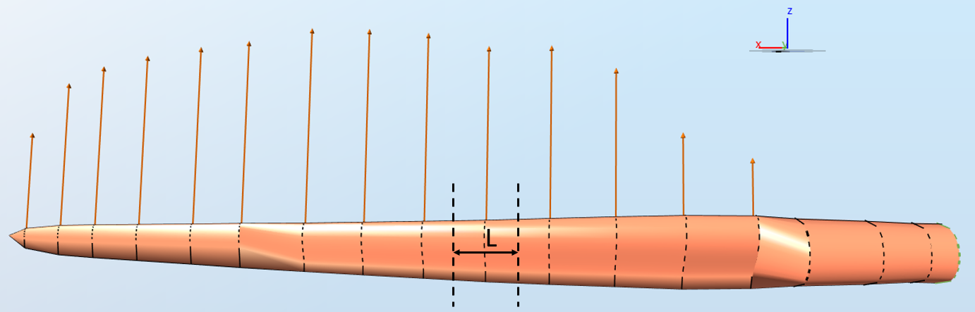
Note: no aerodynamic loads are calculated at the innermost blade aerodynamical station (at the blade root) or the outermost blade aerodynamical station (at the blade tip)
The drag force is applied in the direction of the relative velocity while the lift force is perpendicular to the drag force, as shown in the picture below
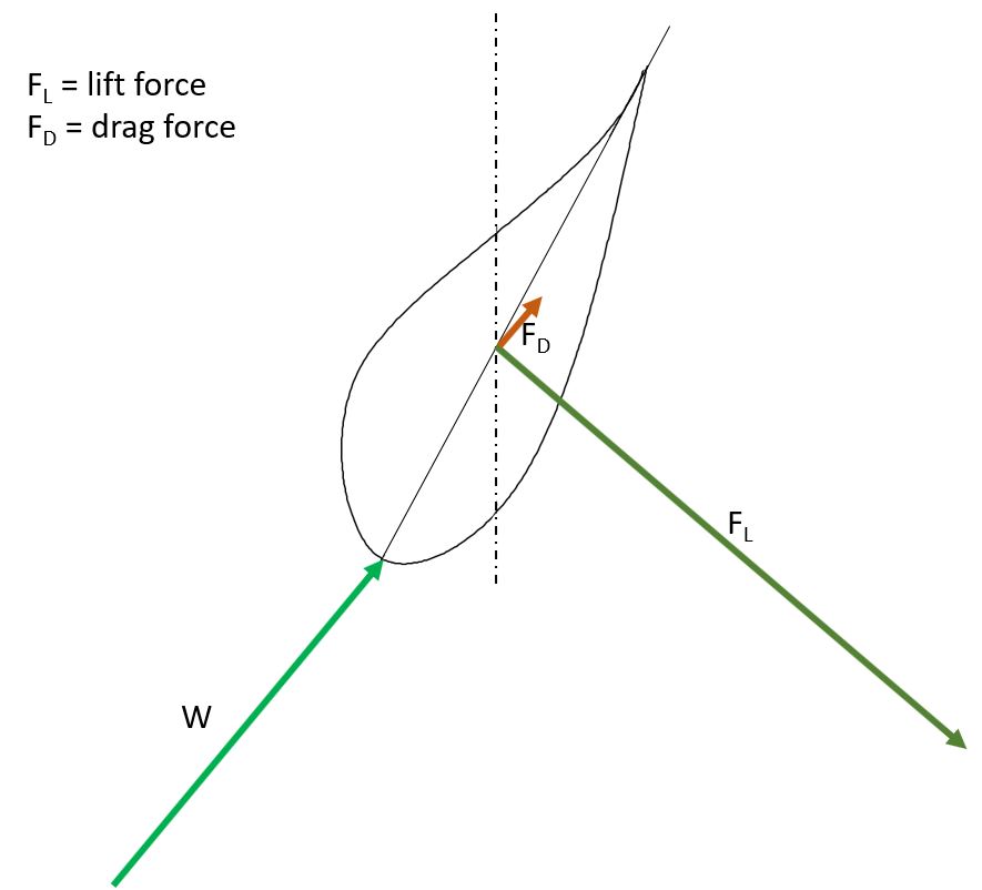
The aerodynamic loads are applied at the aerodynamic center of the displaced blade aerodynamical section
5 Compute the induced velocity
Based on the aerodynamic forces, a new induced velocity can be calculated. A first correction is added at this stage to account for the loss of lift at the tip and at the hub due to the finite number of blades. This correction is called the Prandtl's correction and is given by
$$F_P=F_{tip}\cdot F_{hub}$$
with
$$F_{tip}=\frac{2}{\pi}\cos^{-1}\left[\exp\left({-\frac{N_B}{2}\frac{R-r}{r\sin\phi}}\right)\right]$$
$$F_{hub}=\frac{2}{\pi}\cos^{-1}\left[\exp\left(-\frac{N_B}{2}\frac{r-H_r}{r\sin\phi}\right)\right]$$
where
$$N_B$$
is the number of blades,
$$r$$
is the distance from the blade station to the hub,
$$R$$
is the radius of the rotor,
$$H_r$$
is the radius of the hub and
$$\phi = \alpha + \beta + \theta$$
is the angle between the relative velocity
W and the y-direction. This correction can be toggled on and off in the
Aerodynamics tab of the
Analysis parameters.
The second correction is the so-called
Glauert correction
which accounts for the fact that for heavily loaded rotors (i.e. high values of the axial induction factor), flow recirculation is observed at the back of the rotor and momentum theory breaks down. This is modelled as the
Glauert correction factor
$$A_g$$
, calculated following the
Glauert correction document.
Once these corrections are established, a new induced velocity is computed based on the previous one, following the equation
$$W_{i,new}=\frac{-N_B(F_L\cos\phi+F_D\sin\phi)}{4\pi L\rho rF_PV'}\cdot x -\frac{-N_B(F_L\sin\phi - F_D\cos\phi)}{4\pi L\rho rF_PV'}\cdot y$$
where
$$V'$$
is the wind velocity in the wake, defined as
$$V'=V+A_gn\cdot(W_i\cdot n)$$
with
$$n$$
is the normal to the rotor plane, i.e. the direction of the main shaft of the turbine.6 Compare the induced velocities
Once the new induced velocity has been computed, it is compared to the induced velocity obtained in the previous iteration. If the magnitude of the difference between the two is larger than 1e-8, the iteration is started again from step 2. Otherwise, the algorithm follows to step 7.
7 Yaw/tilt model
When the induced velocity has been established, a correction has to be applied if the wind velocity is not in the rotor normal direction. This correction factor is defined as
$$\Gamma=1+\frac{r}{R}\tan\left(\frac{\chi}{2}\right)\cos(\theta-\theta_0)$$
where
$$\chi$$
is the angle between the velocity in the wake
$$V'$$
and the normal to the rotor plane
$$n$$
,
$$\theta$$
is the azimuth of the blade and
$$\theta_0$$
is the azimuth angle where the blade is the deepest into the wake. In the example given in the figure below, the turbine has no tilt but is yawed 45 degrees. If the azimuth angle is 0 when the blade is pointing upwards, the blade will be the deepest into the wake after 3/4 of a revolution, so
$$\theta_0=270$$
degrees.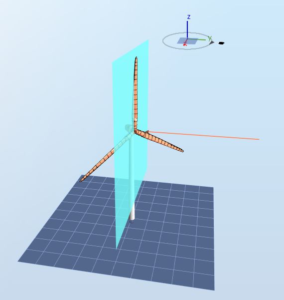
The corrected induced velocity then becomes
$$W_{ic} = W_i\cdot\Gamma$$
8 Compute the aerodynamic loads
Once the current induced velocity is calculated, the angle of attack is computed following step 2, the aerodynamic coefficients are looked up following step 3 and the aerodynamic loads are computed following step 4. In addition to the lift and drag forces, a
pitching moment is calculated following the equation
$$M_p = \frac{1}{2}\rho W^2C^2L$$
The pitching moment is applied around the pitch axis