Eigenmodes
Ashes gives the possibility to perform an eigenfrequency analysis of any model. This video shows how to carry out the analysis for the default onshore wind turbine:
https://www.youtube.com/watch?v=kozASqrgy_o
To carry out an eigenfrequency analysis of a model, select
Eigenmodes in the
View dropdown menu of the
Simulation window (shown in the picture below).

This will open the
eigenmodes
window, which is illustrated below
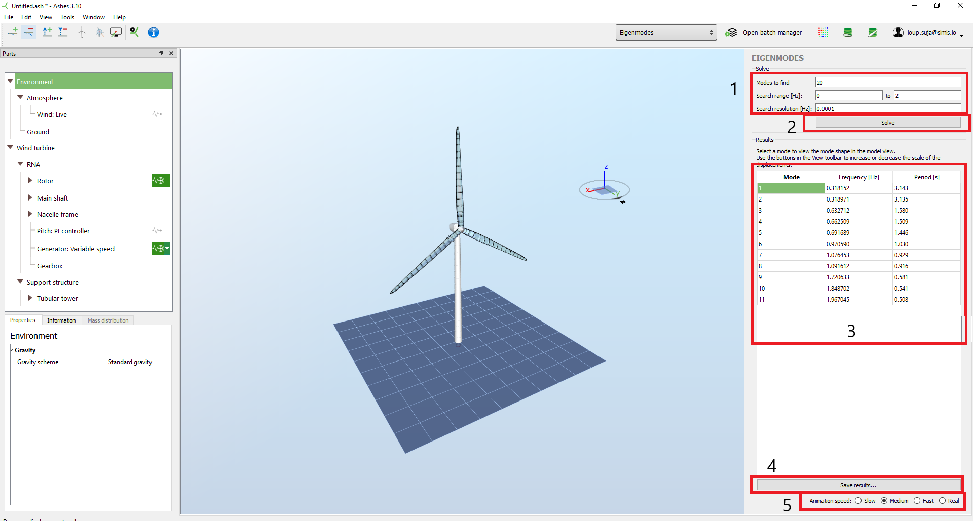
The window has two tabs:
Mode shapes, which lists the natural frequencies of the model and animates each mode, and
Campbell diagram, which plots those frequencies against rotor speed. Both are produced by the same
Solve button, so one press updates both tabs.
The theory behind the two tabs is described in the
Eigenvalue analysis and
Campbell diagram pages of the Theory Manual.
1 Mode shapes
This tab contains the
Parts
and the
Properties panes as the
Simulation window, but includes new elements that are listed and defined below:
- Eigenmodes search definition: these fields enable you to define the parameters of the eigenmodes search. You can define the number of modes to find, the range (in Hz) in which modes are to be found and the resolution, which defines the minimum frequency difference between two successive modes. In the present example, the 1st and 2nd modes (corresponding to fore-aft and side-to-side tower modes) are relatively close. A low search resolution is therefore necessary to ensure that both modes are found.
- Solve button: when this button is pressed, the search of the eigenmodes begins. For complex structures, or if many modes are requested, this search can take up to some minutes. In this case a pop-up window shows the progress of the search.
- Result: this table provides the results in terms of mode number, corresponding frequency (in Hz and in rad/s) and period (in s). If Rayleigh damping is set for the model, an additional Damping ratio column shows the damping ratio associated with each mode's frequency; the column is not shown when the model has no structural damping. You can select any line of this table to visualize the motion of the corresponding mode shape in the main window.
- Save button: pressing this button will save the results to a text file. This also gives the possibility to export the shape of each mode. A mode shape is defined by 9 columns: the first three columns give the initial x-, y- and z-coordinates of each node of the model, the next 3 columns give the x-, y- and z-translations of each node and the last 3 columns give the rotation around the x-, y- and z-axis for each node
- Animation speed: here you can select different options for the speed of the animation of the eigenmodes
Note: the mode shapes exported in the text file are normalised against the
largest displacement obtained for all the degrees of freedom of the system
Note: the frequencies themselves are
undamped natural frequencies — damping does not enter the eigenvalue problem, and the damping ratio in the table is derived from each mode's frequency afterwards. See
Eigenvalue analysis.
If you save the eigenmodes file, you can then use it as one of the
Initial conditions of your simulations. Note that if you select the eigenmodes file as an initial condition, save the model and then delete the file, Ashes will ignore those initial conditions.
2 Campbell diagram
The
Campbell diagram tab plots the natural frequencies of the model against rotor speed, together with the
per-rev excitation lines. It is used to check whether a rotor speed in the operating range excites one of the structure's natural frequencies: a resonance is a point where a mode line crosses a per-rev line.
2.1 Settings
The settings live in the
Campbell box of the control column, next to the
Modes box. They take effect the next time you press
Solve.
| Setting | Description |
|---|---|
| Per-rev lines |
Comma-separated list of the per-rev harmonics to draw, for example
1,3,6. 1 is the rotor's own rotation frequency (1P) and the blade count is the blade-passing frequency (3P for a three-bladed rotor). The field is filled in from the blade count of your model the first time a model is solved, and left alone afterwards. |
| Include rotational effects | When unticked, the diagram simply draws the frequencies of the results table as horizontal lines. When ticked, pressing Solve also runs a full modal analysis at each of a series of rotor speeds, so that blade modes move with rotor speed - flapwise ones curving up steeply, edgewise ones staying nearly flat. |
| Max rotor speed [rpm] | Upper bound of the rotor-speed axis. This applies whether or not rotational effects are included, since it also sets how far the per-rev lines are drawn. Leave it at Auto to use 1.2 times the rated rotor speed of the model (or 15 rpm if the rated speed is unknown). The rated rotor speed is taken from the generator: it is the generator's rated speed divided by the gearbox ratio, so a model whose generator is set to None or to an external controller has no rated speed and falls back to 15 rpm. |
| RPM step [rpm] | Spacing of the rotor speeds actually solved. Only enabled when Include rotational effects is ticked. A smaller step gives smoother curves but more modal solves. Leave it at Auto for about 15 rotor speeds across the range. |
Every rotor speed is a complete modal analysis of the model, so a rotating sweep is much slower than a single eigenmode search. Start with the
Auto step and refine only if you need to resolve a crossing precisely. The sweep shows a progress dialog and can be cancelled at any point.
2.2 Reading the diagram
Example Campbell diagram, with rotating blade modes shown as backward and forward whirl pairs:
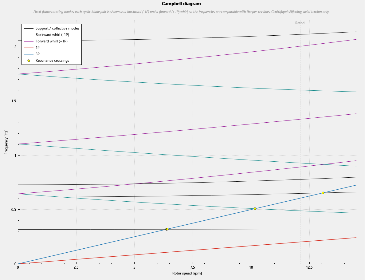
Rotor speed is on the horizontal axis and frequency on the vertical axis. The straight lines through the origin are the per-rev lines; the other lines are the modes. A vertical marker labelled
Rated is drawn at the rated rotor speed of the model, so you can see at a glance which crossings fall inside the operating range; it is omitted when the rated speed is unknown or lies beyond the axis. You can drag and scroll to pan and zoom.
Note: if the rotor-speed axis reaches far higher speeds than your turbine can turn, the model's rated rotor speed is wrong rather than the diagram. This happens when a generator carries a rated speed meant for the high-speed shaft while the model is direct drive, so nothing divides it down - a rated speed of, say, 1174 rpm then puts the axis at about 1400 rpm instead of a few tens. Correct the generator's rated speed, or set
Max rotor speed explicitly instead of leaving it at
Auto.
With rotational effects included, the mode lines are given in the
fixed (ground) frame, which is the frame the per-rev lines belong to, so a crossing between the two really is a resonance. The legend distinguishes three kinds of line:
- Support / collective modes — tower and foundation modes, and blade modes in which all blades move in phase. These are seen at the same frequency from the ground as in the rotor.
- Backward whirl (-1P) and Forward whirl (+1P) — a blade mode in which the blades move out of phase does not appear from the ground at the frequency it has in the blade. It appears as two lines, one 1P below and one 1P above. The backward-whirl line descends as rotor speed increases, even though the blade itself is stiffening.
So one blade family typically produces
three lines: collective, backward whirl and forward whirl. A line drawn
dashed is one Ashes could not convert with full confidence — a blade mode whose whirling partner was not among the modes found, or a backward whirl whose frequency fell below zero and is plotted as its magnitude. Finding more modes often removes the dashes.
The subtitle under the plot title always states which of these cases you are looking at. If the blades of your model cannot be classified — for example if they are not meshed identically — the conversion is skipped, the subtitle says so, and the frequencies are drawn exactly as solved. In that case blade lines are 1P away from what the per-rev lines apply to and crossings should not be read as resonances.
Note: the diagram shows the modes that correspond to the ones in the
Mode shapes results table, so the two tabs cover the same modes. Increase
Modes to find or widen the
Search range to see more lines. Do not expect the
frequencies to match exactly at 0 rpm, though: a pair of whirling blade modes is listed twice in the results table, at two slightly different frequencies, but the diagram averages the pair and draws both lines from that mean. See
Campbell diagram in the Theory Manual for why the mean is the more meaningful number.
2.3 Saving the diagram
Two buttons below the
Solve button export the diagram:
- Save Campbell plot… writes the diagram as an image. The title and subtitle are included, so the exported picture states on its face which frame the frequencies are in.
- Save Campbell data… writes the underlying numbers as a semicolon-separated CSV file.
In the CSV, the first column is the rotor speed and there is one column per mode line. Whirl lines are tagged in the column header, and a header comment states which frame the frequencies are in:
# Rotating modes (centrifugal stiffening and softening; no Coriolis).
# Frequencies are in the fixed (ground) frame, so they can be compared with the per-rev
# lines: each cyclic blade pair appears as a backward whirl (BW, mean - 1P) and a forward
# whirl (FW, mean + 1P). ...

Rotor speed [rpm];Mode 1 [Hz];Mode 2 BW [Hz];Mode 3 FW [Hz];Mode 4 [Hz]
0;0.3179;0.6443;0.6443;0.7561
5;0.3180;0.5655;0.7321;0.7575
A column headed
APPROXIMATE is one of the dashed lines described above. An
empty cell means that line has no value at that rotor speed.2.4 Generating the diagram in batch
The same diagram can be produced without opening the Eigenmodes window, which is useful when you want it for every model in a batch. Tick
Generate Campbell diagram in the
Analysis parameters. The diagram is then computed before the simulation starts and written to
CampbellDiagram.csv in the results folder, in the same format as the interactive export.| Parameter | Description |
|---|---|
| Generate Campbell diagram | Enables the computation. Off by default. |
| Number of eigenmodes to find | How many modes are computed at each rotor speed. Shared with the ordinary batch eigenmode analysis. |
| Campbell max rotor speed | Upper bound of the rotor-speed axis, in rpm. Set it to 0 to derive it as 1.2 times the rated rotor speed, as the Auto setting does in the interactive diagram. |
| Campbell rotor speed step | Spacing of the evaluated rotor speeds, in rpm. Set it to 0 for about 15 rotor speeds across the range. |
Note: rotation is modelled both through the centrifugal
stiffening of the blades and through the centrifugal
softening that cancels most of it again for motion in the plane of rotation. Flapwise and edgewise modes therefore behave differently, as they should: flapwise lines curve up with rotor speed, edgewise lines stay nearly flat. Coriolis and gyroscopic effects are
not included, so the frequencies carry a small high bias and the diagram cannot say whether a resonance it finds is damped. See the
Campbell diagram page of the Theory Manual for the full list of assumptions.