$$L/2$$
comes from the fact that the Morison load affecting an element is split into two equal contributions and applied to each of the nodes composing the element.Morison loads on monopile
This test checks that the sensors corresponding to different terms in the Morison equation output the expected values.
1 Test description
This test uses the default monopile only template in Ashes. The following four load cases are run combining fixed and moving infinitely rigid cylinder in waves as well as current.
-
LC1 Fixed cylinder, wave height
$$H=5\text{ m}$$and wave period$$T = 10\text{ s}$$, no current.
-
LC2. No waves or current, cylinder oscillating horizontally with a period
$$T = 6\text{ s}$$and an amplitude$$A = 2\text{ m}$$
- LC3. Combination of the two above load cases
-
LC4. LC3 with a uniform current with speed
$$c=1.5\text{ m}\cdot\text{s}^{-1}$$
2 Model
The model is illustrated in the figure below.
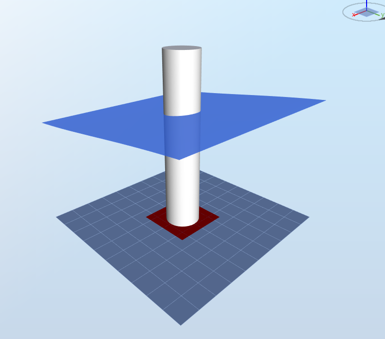
It has a diameter
$$D = 6\text{ m}$$
and is divided into elements of length
$$L=5\text{ m}$$
. For this test, we compute the hydrodynamic loads on the element defined by the nodes at vertical coordinates
$$z_1=-10\text{ m}$$
and
$$z_2=-5\text{ m}$$
. As explained in the
Morison equation document, the fluid kinematics used for computing the Morison loads on an element are taken at the mid-point of the element, hereby corresponding to
$$z_m=-7.5\text{ m}$$
.
The gravitational acceleration is equal to
$$g=9.80665\text{ m}\cdot\text{s}^{-2}$$
and the water density is
$$\rho = 1026.9\text{ kg}\cdot\text{m}^{-3}$$
.
The coefficients for the Morison equation are
$$C_D=1.2$$
and
$$C_M=1.63$$
. Thus
$$C_a = C_M-1=0.63$$
. The water depth is
$$h=-20\text{ m}$$
.3 Analytical results
For each test, we first compute the water velocity and acceleration, including the effect of curent and computed at the horizontal coordinate of the monopile
$$x$$
. Assuming Airy theory in finite water depth, these are given by
$$u(z,x,t) = \omega\frac{H}{2}\frac{\cosh\left(k(z+h)\right)}{\sinh(kh)}\sin(\omega t-kx)+c$$
$$a(z,x,t) = \omega^2\frac{H}{2}\frac{\cosh\left(k(z+h)\right)}{\sinh(kh)}\cos(\omega t-kx)$$
where
$$\omega=2\pi/T$$
and the wave number
$$k$$
is given by the dispersion relationship
$$\omega^2=kg\tanh{kh}$$
The hydrodynamic loads applied to each node are then computed as explained in the
Morison equation document. The loads are split into three components:
- the drag force
$$F_{D}(t) = \rho C_DR\frac{L}{2}\mid u(z_m)-\dot x) \mid(u(z_{m})-\dot x) $$
- the inertia force
$$F_I=\rho C_M\pi R^2\frac{L}{2}a(z_{m}) $$
- the added-mass force
$$F_{a} = -\rho(C_M-1)\pi R^2\frac{L}{2}\ddot x$$
Note: the factor
Note: the added-mass force is not applied as an external force but rather by modifying the mass of the model. The name for such forces in the sensor list will contain the word 'pseudo' to reflect this fact. More information can be found in the
Morison equation document.
4 Results
A simulation of 20 seconds is run for each load case. The results are considered passed if the results from Ashes are within 2% of the analytical solution.
The report for this test can be found on the following link: