Y-Joints Stresses
This document describes a verification test where the results from Ashes are compared to the analytical solution for stresses in a tubular joint according to DNV RP-C203.
1 Test Description
We define a joint and apply a load in a given direction. The stress concentration factors (SCFs) are hardcoded. For each physical Y joint, we define two joint sensors: one for the brace side and one for the chord side. This makes it possible to get different stresses on either side. For each joint sensor, we define 4 SCFs:
- SCF_AS: Axial stress concentration factor at saddle
- SCF_AC: Axial stress concentration factor at crown
- SCF_MIP: In-plane bending stress concentration factor
- SCF_MOP: Out-of-plane bending stress concentration factor
We then apply a load and compute the stress around 8 points based on DNV RP-C203.
Note: a positive stress means tension, and a negative stress means compression
2 Analytical Solution
Stresses at the 8 circumferential points of each sensor are computed following the description in the
Fatigue document.
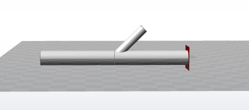
3 Test 1: Y-Joint with Vertical Load
3.1 Model Configuration
The Y-joint is defined with the following nodes:
| Node | X (m) | Y (m) | Z (m) |
|---|---|---|---|
| A | 0 | 0 | 0 |
| B | 10 | 0 | 0 |
| C | 3 | 0 | 2 |
| D | 5 | 0 | 0 |
The brace (member DC) has a circular hollow cross section with:
- Diameter: $$D = 0.6$$m
- Thickness: $$t = 0.03$$m
The chord (members AD and DB) has a circular hollow cross section with:
- Diameter: $$D = 1.0$$m
- Thickness: $$t = 0.05$$m
Two joint sensors are defined:
- Brace side: SCF_AS = 4, SCF_AC = 2, SCF_MIP = 3, SCF_MOP = 5
- Chord side: SCF_AS = 6, SCF_AC = 3, SCF_MIP = 4, SCF_MOP = 6
A vertical load of
$$F = 80\,000$$
N is applied downwards on node C.
The model is shown in the figure below:
3.2 Cross-Sectional Area and Second Moment of Area
The cross-sectional area of the brace is:
$$A = \frac{\pi}{4}\left(D^2 - (D - 2t)^2\right) = 0.05372 \text{ m}^2$$
The second moment of area of the brace is:
$$I =\frac{\pi}{64}\left(D^4 - (D - 2t)^4\right) = 0.002188 \text{ m}^4$$
3.3 Axial and Bending Stress
The brace member DC runs from D = (5, 0, 0) to C = (3, 0, 2), giving a length of
$$L = \sqrt{(5-3)^2 + (0-0)^2 + (0-2)^2} = 2\sqrt{2} \approx 2.828$$
m. The member is oriented at 45° from the horizontal chord, so the vertical load of 80 000 N decomposes into an axial component and a transverse component along the brace local axes. The axial force in the brace is:
$$N = -F \cdot \frac{\sqrt{2}}{2} = -80\,000 \cdot \frac{\sqrt{2}}{2} \approx -56\,568.5 \text{ N}$$
The corresponding axial stress is:
$$\sigma_x = \frac{N}{A} = \frac{-56\,568.5}{0.05372} \approx -1.053 \text{ MPa}$$
The transverse component of the load (perpendicular to the brace axis, in the XZ plane) is:
$$V = F \cdot \frac{\sqrt{2}}{2} = 80\,000 \cdot \frac{\sqrt{2}}{2} \approx 56\,568.5 \text{ N}$$
This transverse force produces an in-plane bending moment at the joint end of the brace. The brace length is
$$L = 2.828$$
m, so the bending moment at the fixed end is:
$$M_y = -V \cdot L = 56\,568.5 \times 2.828 \approx -160 \text{ kN·m}$$
The corresponding in-plane bending stress (evaluated at the outer fibre,
$$c = D/2 = 0.3$$
m) is:
$$\sigma_{my} = \frac{M_y \cdot c}{I} = \frac{-160\,000 \times 0.3}{0.002188} \approx -21.940 \text{ MPa}$$
Since the load is applied in the XZ plane, there is no out-of-plane bending. The input stresses are therefore:
- $$\sigma_x = -1.053$$MPa
- $$\sigma_{my} = -21.940$$MPa
- $$\sigma_{mz} = 0$$MPa
3.4 Expected Stresses at Eight Points
Using the SCFs and input stresses defined above, the stresses at the eight circumferential positions are:
| Point | Brace Side (MPa) | Chord Side (MPa) |
|---|---|---|
$$\sigma_0$$ |
-67.93 | -90.92 |
$$\sigma_{45}$$ |
-49.70 | -66.79 |
$$\sigma_{90}$$ |
-4.21 | -6.32 |
$$\sigma_{135}$$ |
43.38 | 57.32 |
$$\sigma_{180}$$ |
63.71 | 84.60 |
$$\sigma_{225}$$ |
43.38 | 57.32 |
$$\sigma_{270}$$ |
-4.21 | -6.32 |
$$\sigma_{315}$$ |
-49.70 | -66.79 |
4 Test 2: Y-Joint with Horizontal Load in Y-Direction
4.1 Model Configuration
The model geometry, cross-sections, and joint sensor SCFs are identical to those defined in Section 3.1 and 3.2. A horizontal load of
$$F_y = 40\,000$$
N is applied in the positive Y-direction on node C.
4.2 Axial and Bending Stress
The load is applied in the Y-direction, which is perpendicular to the plane containing the brace and chord (the XZ plane). The brace axis lies entirely in the XZ plane, so the Y-direction load produces no axial force in the brace. The load acts as a purely out-of-plane transverse force on the brace, generating an out-of-plane bending moment at the joint end. The bending moment at the fixed end is:
$$M_z = F_y \cdot L = 40\,000 \times 2.828 \approx 113\,137 \text{ N·m}$$
The corresponding out-of-plane bending stress (evaluated at the outer fibre,
$$c = D/2 = 0.3$$
m) is:
$$\sigma_{mz} = \frac{M_z \cdot c}{I} = \frac{113\,137 \times 0.3}{0.002188} \approx 15.513 \text{ MPa}$$
The input stresses are therefore:
- $$\sigma_x = 0$$MPa
- $$\sigma_{my} = 0$$MPa
- $$\sigma_{mz} = 15.513$$MPa
4.3 Expected Stresses at Eight Points
Using the SCFs and input stresses defined above, the stresses at the eight circumferential positions are:
| Point | Brace Side (MPa) | Chord Side (MPa) |
|---|---|---|
$$\sigma_0$$ |
0.000 | 0.000 |
$$\sigma_{45}$$ |
-54.85 | -65.82 |
$$\sigma_{90}$$ |
-77.57 | -93.08 |
$$\sigma_{135}$$ |
-54.85 | -65.82 |
$$\sigma_{180}$$ |
0.000 | 0.000 |
$$\sigma_{225}$$ |
54.85 | 65.82 |
$$\sigma_{270}$$ |
77.57 | 93.08 |
$$\sigma_{315}$$ |
54.85 | 65.82 |
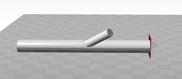
5 Test 3: Y-Joint Rotated 45° About X-Axis with Combined Load
5.1 Model Configuration
This test uses the same model as Test 2 (Section 4), but with the structure rotated 45° about the X-axis. The node positions are identical to those in Section 3.1, except for node C which now has coordinates:
| Node | X (m) | Y (m) | Z (m) |
|---|---|---|---|
| A | 0 | 0 | 0 |
| B | 10 | 0 | 0 |
| C | 3 | 1.414 | 1.414 |
| D | 5 | 0 | 0 |
In order to keep the applied load oriented in the same direction relative to the joint (i.e., equivalent to the Y-direction load of Test 2 after the rotation), the load is applied as:
$$\mathbf{F} = \left(0,\; 28\,284,\; -28\,284\right) \text{ N}$$
This load vector corresponds to a rotation of the 40 000 N Y-direction load by 45° about the X-axis, and is therefore physically equivalent to the loading in Test 2.
The model is shown in the figure below>:
5.2 Expected Results
Since this test is a rigid-body rotation of Test 2, all sectional stresses and resulting circumferential stresses at the joint are identical to those reported in Section 4.3. No additional computation is required.
6 Test 4: Y-Joint with Combined 3D Load
6.1 Model Configuration
The model geometry, cross-sections, and joint sensor SCFs are identical to those defined in Section 3.1. The cross-sectional properties of the brace are also the same as derived in Section 3.2:
- Cross-sectional area: $$A = 0.05372 \text{ m}^2$$
- Second moment of area: $$I = 0.002188 \text{ m}^4$$
- Brace length: $$L = 2\sqrt{2} \approx 2.828 \text{ m}$$
The applied load on node C is now a combined three-dimensional force:
$$\mathbf{F} = \left(30\,000,\; 40\,000,\; 20\,000\right) \text{ N}$$
6.2 Axial and Bending Stress
The brace member DC runs from D = (5, 0, 0) to C = (3, 0, 2). The unit vector along the brace axis (from D to C) is:
$$\hat{\mathbf{e}}_x = \frac{1}{2\sqrt{2}}\left(-2,\; 0,\; 2\right) = \left(-\frac{\sqrt{2}}{2},\; 0,\; \frac{\sqrt{2}}{2}\right)$$
The axial force in the brace is the projection of the applied force onto the brace axis:
$$N = \mathbf{F} \cdot \hat{\mathbf{e}}_x = 30\,000 \cdot \left(-\frac{\sqrt{2}}{2}\right) + 40\,000 \cdot 0 + 20\,000 \cdot \frac{\sqrt{2}}{2} = -\frac{\sqrt{2}}{2} \cdot 10\,000 \approx -7\,071.1 \text{ N}$$
The corresponding axial stress is:
$$\sigma_x = \frac{N}{A} = \frac{-7\,071.1}{0.05372} \approx -0.1316 \text{ MPa}$$
The transverse force vector (perpendicular to the brace axis) is:
$$\mathbf{V} = \mathbf{F} - N \cdot \hat{\mathbf{e}}_x = \left(30\,000,\; 40\,000,\; 20\,000\right) - (-7\,071.1)\cdot\left(-\frac{\sqrt{2}}{2},\; 0,\; \frac{\sqrt{2}}{2}\right)$$
$$\mathbf{V} = \left(30\,000 - 5\,000,\; 40\,000,\; 20\,000 + 5\,000\right) = \left(25\,000,\; 40\,000,\; 25\,000\right) \text{ N}$$
The brace local coordinate system has its x-axis along
$$\hat{\mathbf{e}}_x$$
. The local y-axis lies in the XZ plane (the plane of the brace and chord), perpendicular to the brace axis. The local z-axis is perpendicular to the XZ plane (i.e., along the global Y-direction). Specifically:
- Local y-axis (in-plane): $$\hat{\mathbf{e}}_y = \left(\frac{\sqrt{2}}{2},\; 0,\; \frac{\sqrt{2}}{2}\right)$$
- Local z-axis (out-of-plane): $$\hat{\mathbf{e}}_z = \left(0,\; 1,\; 0\right)$$
The in-plane transverse force (producing in-plane bending moment
$$M_y$$
) is:
$$V_y = \mathbf{V} \cdot \hat{\mathbf{e}}_y = 25\,000 \cdot \frac{\sqrt{2}}{2} + 40\,000 \cdot 0 + 25\,000 \cdot \frac{\sqrt{2}}{2} = 50\,000 \cdot \frac{\sqrt{2}}{2} \approx 35\,355.3 \text{ N}$$
The out-of-plane transverse force (producing out-of-plane bending moment
$$M_z$$
) is:
$$V_z = \mathbf{V} \cdot \hat{\mathbf{e}}_z = 25\,000 \cdot 0 + 40\,000 \cdot 1 + 25\,000 \cdot 0 = 40\,000 \text{ N}$$
The bending moments at the joint end of the brace are:
$$M_y = V_y \cdot L = 35\,355.3 \times 2.828 \approx 99\,987 \text{ N·m}$$
$$M_z = V_z \cdot L = 40\,000 \times 2.828 \approx 113\,137 \text{ N·m}$$
The corresponding bending stresses (evaluated at the outer fibre,
$$c = D/2 = 0.3$$
m) are:
$$\sigma_{my} = \frac{M_y \cdot c}{I} = \frac{99\,987 \times 0.3}{0.002188} \approx 13.712 \text{ MPa}$$
$$\sigma_{mz} = \frac{M_z \cdot c}{I} = \frac{113\,137 \times 0.3}{0.002188} \approx 15.513 \text{ MPa}$$
The input stresses are therefore:
- $$\sigma_x = -0.1316$$MPa
- $$\sigma_{my} = 13.712$$MPa
- $$\sigma_{mz} = 15.513$$MPa
6.3 Expected Stresses at Eight Points
Using the SCFs and input stresses defined above, the stresses at the eight circumferential positions are computed using the formulas in Section 2.1.3. The results are:
| Point | Brace Side (MPa) | Chord Side (MPa) |
|---|---|---|
$$\sigma_0$$ |
40.87 | 54.45 |
$$\sigma_{45}$$ |
-26.16 | -27.63 |
$$\sigma_{90}$$ |
-78.10 | -93.87 |
$$\sigma_{135}$$ |
-84.22 | -105.20 |
$$\sigma_{180}$$ |
-41.40 | -55.24 |
$$\sigma_{225}$$ |
25.37 | 26.44 |
$$\sigma_{270}$$ |
77.04 | 92.29 |
$$\sigma_{315}$$ |
83.54 | 104.01 |
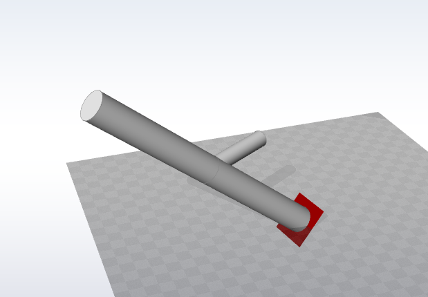
7 Test 5: Y-Joint Rotated [30°, −40°, 10°] About Node A with Combined Load
7.1 Model Configuration
This test uses the same loading scenario as Test 4 (Section 6), but with the entire structure rotated sequentially by 30°, −40°, and 10° about the X-, Y-, and Z-axes respectively, with node A as the pivot. The resulting node coordinates are:
| Node | X (m) | Y (m) | Z (m) |
|---|---|---|---|
| A | 0.000 | 0.000 | 0.000 |
| B | 7.544 | 1.330 | 6.428 |
| C | 1.340 | −0.779 | 3.255 |
| D | 3.772 | 0.665 | 3.214 |
To maintain the same loading relative to the joint as in Test 4, the applied force has been rotated by the same transformation, giving:
$$\mathbf{F} = \left(-5\,271,\; 24\,092,\; 47\,873\right) \text{ N}$$
The model is shown in the figure below:
7.2 Expected Results
Since this test is a rigid-body rotation of Test 4, the sectional stresses in the brace local coordinate system are unchanged. All circumferential stresses at the joint are therefore identical to those reported in Section 6.3. No additional computation is required.
8 Test 6: Y-Joint with Sinusoidally Varying Load
8.1 Model Configuration
This test uses the same model as Test 5 (Section 7), including the rotated node coordinates and the same cross-section properties and joint sensor SCFs. The only difference is that the force is now applied sinusoidally in time rather than as a static load. The force amplitude is identical to the static force used in Test 5:
$$\mathbf{F}(t) = \left(-5\,271,\; 24\,092,\; 47\,873\right) \cdot \sin\!\left(\frac{2\pi t}{T}\right) \text{ N}, \quad T = 30 \text{ s}$$
8.2 Expected Results
Because the structural response is linear and the loading is sinusoidal, all sectional stresses and circumferential joint stresses vary sinusoidally in time with the same period
$$T = 30$$
s. The amplitude of each stress component is equal to the corresponding static value reported in Section 6.3. That is, for each circumferential position $$\theta$$
:
$$\sigma_\theta(t) = \hat{\sigma}_\theta \cdot \sin\!\left(\frac{2\pi t}{30}\right)$$
where
$$\hat{\sigma}_\theta$$
is the amplitude, equal to the static stress value at position $$\theta$$
from Section 6.3.
9 Report
A time simulation of 5 seconds is run for each load case and the last 20% are compared to the analytical solution. If the results from Ashes are within 0.5% of the analytical solution, the test is considered passed.
The report of this test can be found on the following link: